What is COLUMNS function in Excel?
The COLUMNS function is one of the Lookup & reference functions of Excel.
It Returns the number of columns in an array or reference.
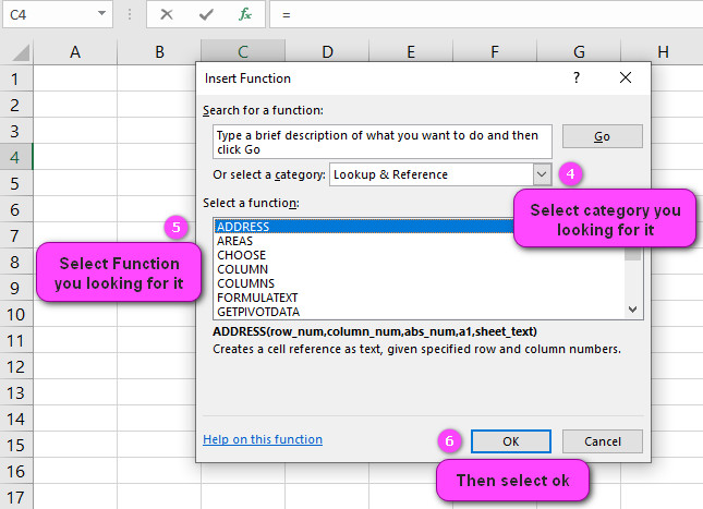
We can find this function in Lookup & reference of insert function Tab.
How to use COLUMNS function in excel
- Click on an empty cell (like F5 ).

2. Click on the fx icon (or press shift+F3).

3. In the insert function tab you will see all functions.

4. Select Lookup & reference category.
5. Select COLUMNS function.
6. Then select ok.
7. In the function arguments Tab, you will see COLUMNS function.
8. Array is an array or array formula, or a reference to a range of cells for which you want the number of columns.
9. For example If you click on A4:G4 , see result= 7.

10. or If you click on A4, see result= 1

11. You will see the result in the formula result section
Examples of COLUMNS function in excel

Discover the Power of Excel’s Columns Function
Excel’s COLUMN function is a powerful tool for working with columns in your worksheets. It returns the column number of a specific cell or range reference and can be used in a variety of ways to manipulate and analyze data. For example, you can use the COLUMN function with other functions like SUM, AVERAGE, and COUNT to create complex formulas that perform calculations across multiple columns.
Example: Suppose you have a worksheet with sales data for different products in columns A through F. You could use the COLUMN function to create a formula that calculates the average sales for all products in columns B through F, like this: “=AVERAGE(B:F)”.
How to Effectively Use Excel’s Columns Function
To effectively use Excel’s COLUMN function, it’s important to understand its syntax and how it works with other functions and formulas. The basic syntax of the COLUMN function is “=COLUMN(reference)”, where “reference” is the cell or range reference you want to return the column number for. You can also use the COLUMN function with other functions like IF, SUMIF, and COUNTIF to create more complex calculations based on column values.
Example: Suppose you have a worksheet with customer information in columns A through D. If column D contains a value of “Yes” for customers who have subscribed to your newsletter, you could use the COUNTIF function with the COLUMN function to count the total number of subscribers in column D like this: “=COUNTIF(D:D, “Yes”)”.
Mastering the Syntax of Excel’s Columns Function
Mastering the syntax of Excel’s COLUMN function is essential for creating effective and efficient formulas. In addition to the basic syntax of “=COLUMN(reference)”, you can also use optional arguments like “col_index_num” to specify the column number you want to return, and “range_reference” to specify the range of cells you want to return the column numbers for. You can also use the COLUMN function with other functions like VLOOKUP, INDEX, and MATCH to perform more complex calculations based on specific columns.
Example: Suppose you have a worksheet with shipping information in columns A through F, and you want to calculate the total shipping cost for each order. You could use the SUM function with the COLUMN function and absolute cell references to create a formula that sums up the values in columns B through F for each row, like this: “=SUM(�2:B2:F2)”.
Select Multiple Columns with Excel’s Columns Function
Excel’s COLUMN function is a useful tool for selecting multiple columns in your worksheets. To select multiple columns using the COLUMN function, you can use the “:” (colon) operator to define a range of columns, or the “,” (comma) operator to specify individual columns. You can also use the COLUMN function with other functions like OFFSET, INDIRECT, and INDEX to create more dynamic and flexible selections based on specific criteria.
Example: Suppose you have a worksheet with product information in columns A through F, and you want to select only the columns for product name, price, and quantity sold. You could use the COLUMN function with the CHOOSE function and the comma operator to select the specific columns, like this: “=CHOOSE({1,2,3},A:A,B:B,C:C)”.
Formatting Text in Excel Columns: Tips and Tricks Using the Columns Function
Formatting text in Excel columns is an important aspect of creating professional-looking worksheets. The Columns function can help you format text more efficiently by allowing you to apply formatting options to entire columns or ranges of columns at once. This includes options like font type, font size, bolding, italicizing, underlining, and more.
Example: Suppose you have a worksheet with customer information in columns A through D, and you want to apply bold formatting to the column headers. You could use the Columns function with the BOLD function to create a formula that applies bold formatting to all cells in rows 1 through 4, like this: “=BOLD(COLUMNS(A:D)&”1:”&COLUMNS(A:D)&”4″)”.
Sorting Data in Excel: Simplified with the Columns Function
Sorting data in Excel is essential for analyzing and organizing your data effectively. The Columns function can simplify the sorting process by allowing you to specify which columns you want to sort and how you want to sort them. This saves time and effort, especially when working with large amounts of data.
Example: Suppose you have a sales report with columns for product names, prices, quantities sold, and revenue, and you want to sort the data based on the revenue column in descending order. You could use the Columns function with the SORT function to create a formula that sorts the data in ascending or descending order, like this: “=SORT(A2:E10,4,-1)”.
Filtering Data in Excel: Quick and Simple with the Columns Function
Filtering data in Excel is an important data analysis function that allows you to quickly and easily display only the data that meets specific criteria. The Columns function can simplify the filtering process by allowing you to specify which columns you want to filter and which criteria you want to apply. This saves time and effort, especially when working with large datasets.
Example: Suppose you have a worksheet with customer information in columns A through D, and you want to filter the data to show only customers who live in a specific region. You could use the Columns function with the FILTER function to create a formula that filters the data based on the region column and the criteria you specify, like this: “=FILTER(A2:D10,C2:C10=”North”)”.
Inserting New Columns in Excel: A Tutorial Using the Columns Function
Inserting new columns in Excel is an important editing function that allows you to add new data or rearrange your existing data more effectively. The Columns function can help you insert new columns quickly and easily by allowing you to specify where you want to insert the new columns and how many columns you want to insert.
Example: Suppose you have a sales report with columns for product names, prices, quantities sold, and revenue, and you want to insert a new column between the Price and Quantity Sold columns for a new data point. You could use the Columns function with the INSERT function to create a formula that inserts a new column at the appropriate position, like this: “=INSERT(B1:F1,2)”.
Deleting Columns in Excel: A Guide Using the Columns Function
Deleting columns in Excel is a common editing function that allows you to remove unnecessary data or rearrange your existing data more effectively. The Columns function can help you delete columns quickly and easily by allowing you to specify which columns you want to delete and how many columns you want to delete.
Example: Suppose you have a sales report with columns for product names, prices, quantities sold, and revenue, and you want to delete the Quantity Sold column because it’s no longer needed. You could use the Columns function with the DELETE function to create a formula that deletes the appropriate column, like this: “=DELETE(C:C)”.
Merging Cells in Excel: The Easiest Way with the Columns Function
Merging cells in Excel is a useful formatting function that allows you to combine multiple cells into a single cell. The Columns function can make merging cells easier by allowing you to select entire columns or ranges of columns and merge them into a single cell or range of cells.
Example: Suppose you have a worksheet with customer information in columns A through D, and you want to merge the header cells in the first row into a single cell. You could use the Columns function with the MERGE function to create a formula that merges the cells into one, like this: “=MERGE(A1:D1)”.
Splitting Cells in Excel: A How-To Guide Using the Columns Function
Splitting cells in Excel is a useful function that allows you to separate data that’s been combined into a single cell into separate cells. The Columns function can help you split cells more efficiently by allowing you to specify where you want to split the data and how many new columns you want to create.
Example: Suppose you have a worksheet with customer information in a single cell in column A, with the name, address, and phone number all combined. You could use the Columns function with the SPLIT function to create a formula that splits the data into separate columns, like this: “=SPLIT(A2,”|”)”.
Renaming Columns in Excel: The Simplest Method with the Columns Function
Renaming columns in Excel is an important editing function that allows you to update the column headers to better reflect the data they contain. The Columns function can help you rename columns more efficiently by allowing you to select entire columns or ranges of columns and apply new names.
Example: Suppose you have a sales report with columns for product names, prices, quantities sold, and revenue, but you want to change the name of the Quantity Sold column to Units Sold to better reflect the data. You could use the Columns function with the RENAME function to create a formula that renames the appropriate column, like this: “=RENAME(C:C,”Units Sold”)”.
Copying and Pasting Data in Excel: Streamlined with the Columns Function
Copying and pasting data in Excel is a common editing function that allows you to replicate or move data within your worksheet. The Columns function can help streamline this process by allowing you to select entire columns or ranges of columns and copy them quickly and easily.
Example: Suppose you have a sales report in columns A through D, and you want to copy the data in columns B and C to a new location in your worksheet. You could use the Columns function to select those columns and the COPY function to create a formula that copies them to a new location, like this: “=COPY(B:C)”.
Transposing Data in Excel: A Comprehensive Guide Using the Columns Function
Transposing data in Excel is a useful function that allows you to reorganize your data from rows into columns or vice versa. The Columns function can help with this process by allowing you to select entire rows or ranges of rows and transpose them quickly and easily.
Example: Suppose you have a sales report in rows 2 through 6, with product names in column A and sales data in columns B through F. If you want to transpose the data so that the product names are in row 1 and the sales data is in columns A through E, you could use the Columns function with the TRANSPOSE function to create a formula that transposes the data, like this: “=TRANSPOSE(A2:F6)”.
Unlocking the Full Potential of Excel’s Columns Function for Calculations
Excel’s COLUMN function is a powerful tool for performing calculations across multiple columns in your worksheets. To unlock its full potential, it’s important to understand its syntax and how it works with other functions and formulas. By using the Columns function with other functions like SUM, AVERAGE, and COUNT, you can create complex formulas that perform calculations across entire ranges of columns.
Example: Suppose you have a sales report with columns for product names, prices, quantities sold, and revenue. You could use the Columns function with the SUM function to create a formula that calculates the total revenue generated by all products in all regions, like this: “=SUM(B:F)”.
Exploring Excel’s Columns Function: What You Need to Know
Excel’s COLUMN function is a versatile tool for working with columns in your worksheets. By returning the column number of a specific cell or range reference, it can be used in a variety of ways to manipulate and analyze data. Understanding its syntax and how it works with other functions and formulas is essential for unlocking its full potential.
Example: Suppose you have a worksheet with customer information in columns A through D. If column D contains a value of “Yes” for customers who have subscribed to your newsletter, you could use the COUNTIF function with the COLUMN function to count the total number of subscribers in column D like this: “=COUNTIF(D:D, “Yes”)”.
COLUMNS related functions
- COLUMN function
- ROW function
- ROWS function
- FILTER function

