Excel XMATCH Function

What is XMATCH function in Excel?

The XMATCH function is one of the Lookup & reference functions of Excel.

It searches a range or an array for a match and returns the corresponding item from a second range or array.

By default , an exact match mode is used.

We can find this function in Lookup & reference category of insert function Tab.

How to use XMATCH function in excel

1. Click on an empty cell (like F5).

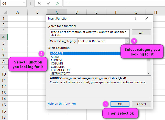
2. Click on the fx icon (or press shift+F3).

3. In the insert function tab you will see all functions.

4. Select Lookup & reference category.

5. Select XMATCH function

6. Then select ok.

7. In function arguments Tab, you will see XMATCH function.

8. Lookup value is the value to search for.

9. Table_array is the array or range to search.

10. Return_array is the array or range to return .

11. If_not_found is returned if no match is found.

12. Match_mode specifies how to match lookup_value against the values in lookup_array.

13. You will see the result in the formula result section.

Examples of XMATCH function in excel

Here are some examples of how to use the XMATCH function in Excel:

1. Exact match: Suppose you have a list of numbers in column A, and you want to find the position of the number 10 in the list. You can use the following formula using XMATCH:

=XMATCH(10,A:A,0)

This formula will return the position of the cell in column A that contains the value 10.

2. Approximate match: Suppose you have a list of prices in column A, and you want to find the position of the price that is closest to $5.50.
   • You can use the following formula using XMATCH with match_mode set to -1 (exact match or next smaller value):

=XMATCH(5.5,A:A,-1)

This formula will return the position of the cell in column A that contains the value closest to $5.50.

3. Lookup based on pattern: Suppose you have a list of names in column A, and you want to find the first name that starts with the letter “J”.
   • You can use the following formula using XMATCH with match_mode set to 2 (wildcard match) and “J*” as the lookup_value:

=XMATCH(“J*”,A:A,2)

This formula will return the position of the first cell in column A that contains a name starting with the letter “J”.

4. Using XMATCH with arrays: Suppose you have a list of product IDs in column A and their corresponding prices in column B, and you want to retrieve the prices for a list of product IDs in cells D1:D5. You can use the following formula:

=XMATCH(D1:D5,A:A,B:B)

This formula will return an array of the same size as the input array, containing the positions of the matching rows in column A.

You can then use these positions to extract the corresponding prices from column B using the INDEX function.

5. Handling errors: Suppose you have a list of numbers in column A, and you want to find the position of the number 1000 in the list.
   • However, 1000 is not in the list. You can use the following formula to handle the resulting #N/A error:

=IFERROR(XMATCH(1000,A:A,0), “Not found”)

This formula will first attempt to use XMATCH to find the position of 1000 in column A. If it fails (due to not finding a match), it will return the message “Not found” instead of the error value.

These are just a few examples of how to use the XMATCH function in Excel. By combining XMATCH with other functions and techniques, you can perform more complex calculations and manipulations on your data.

How is the XMATCH function different from the MATCH function in Excel?

The XMATCH function in Excel is a newer and more powerful version of the MATCH function.

While both functions can be used to find the position of an item in a range of cells, there are some key differences.

1. Return Type: The primary difference between the two functions is that the MATCH function always returns an exact match (i.e., it only returns the position of the first cell that matches the lookup value exactly), whereas the XMATCH function can return either an exact match or an approximate match.
2. Match Mode: The XMATCH function has four different match modes to choose from: 0 (exact match), -1 (exact match or next smaller value), 1 (exact match or next larger value), and 2 (wildcard match).
   • This means that you can use the XMATCH function to perform approximate matches, which can be very useful when working with large datasets or when dealing with data that is not perfectly clean.

Here are some examples to illustrate the differences between the two functions:

Example 1: Suppose we have a list of names in column A and corresponding scores in column B.

We want to use the MATCH function to find the position of “John” in column A.

=MATCH(“John”,A:A,0)

This formula will return the position of the first cell in column A that exactly matches “John”.

However, if “John” is not found in column A, it will return an error value (#N/A).

Now, let’s use the XMATCH function to achieve the same result:

=XMATCH(“John”,A:A,0)

This formula will also return the position of the first cell in column A that exactly matches “John”. However, if “John” is not found in column A, it will return the error value #VALUE!.

Example 2: Suppose we have a list of prices in column A and corresponding products in column B.

We want to use the MATCH function to find the position of the first price that is greater than or equal to $10.

=MATCH(10,A:A,1)

This formula will return the position of the first cell in column A that contains a value greater than or equal to 10.

However, if there is no such value in column A, it will return an error value (#N/A).

Now, let’s use the XMATCH function to perform the same search:

=XMATCH(10,A:A,1)

This formula will return the position of the first cell in column A that contains a value greater than or equal to 10.

If there is no such value in column A, it will return the position of the last cell in column A that contains a value less than 10.

As you can see, the XMATCH function allows for more flexibility and control when searching for values in a range of cells.

By using its different match modes, you can perform exact matches, approximate matches, and even wildcard matches with ease.

What are the syntax and arguments of the XMATCH function in Excel?

Sure! The syntax for the XMATCH function in Excel is as follows:

=XMATCH(lookup_value, lookup_array, [match_mode], [search_mode])

Here’s what each argument means:

1. Lookup_value: This is the value that you want to find in the lookup_array.
2. Lookup_array: This is the range of cells in which you want to search for the lookup_value.
   • It can be a single row or column, or a two-dimensional array.
3. Match_mode (optional): This determines the type of match to perform.
   • There are four possible values:

• 0: Exact match (default)
• -1: Exact match or next smaller value
• 1: Exact match or next larger value
• 2: Wildcard match

4. Search_mode (optional): This determines how the search is conducted.
   • There are two possible values:

• 1: Search from the beginning of the array (default)
• -1: Search from the end of the array

Note that both match_mode and search_mode are optional arguments. If they are not specified, the function will use their default values (0 for match_mode and 1 for search_mode).

Now let’s look at some examples to see how the XMATCH function works:

Example 1: Basic usage Suppose we have a list of numbers in column A, and we want to find the position of the number 5 in this list.

We can use the XMATCH function as follows:

=XMATCH(5,A:A)

This formula will return the position of the first cell in column A that contains the value 5.

Example 2: Approximate match Suppose we have the same list of numbers in column A as before, but this time we want to find the position of the number 4.5 or the closest value that is less than 4.5.

We can use the XMATCH function with match_mode set to -1 (exact match or next smaller value) as follows:

=XMATCH(4.5,A:A,-1)

This formula will return the position of the first cell in column A that contains a value less than or equal to 4.5.

Example 3: Wildcard match Suppose we have a list of fruits in column A, and we want to find the position of the first fruit that starts with the letter “a”.

We can use the XMATCH function with match_mode set to 2 (wildcard match) as follows:

=XMATCH(“a*”,A:A,2)

This formula will return the position of the first cell in column A that contains a fruit whose name starts with the letter “a”.

Overall, the XMATCH function is a powerful and versatile tool for finding values in a range of cells, and its various match modes make it even more flexible and useful.

In which situations should I use the XMATCH function instead of the MATCH function in Excel?

There are several situations in which you should use the XMATCH function instead of the MATCH function in Excel:

1. When performing approximate matches: The XMATCH function allows you to perform approximate matches by specifying a match_mode other than 0 (exact match).
   • This can be useful when working with large datasets or when dealing with data that is not perfectly clean.

For example, if you have a list of prices and you want to find the first price that is greater than or equal to $10, you can use the XMATCH function with match_mode set to 1 (exact match or next larger value):

=XMATCH(10,A:A,1)

This formula will return the position of the first cell in column A that contains a value greater than or equal to 10.

2. When searching for values in unsorted arrays: The XMATCH function can search for values in unsorted arrays using the search_mode argument. By setting search_mode to -1 (search from the end of the array), you can search for values in reverse order, which can be useful in some cases.

For example, if you have a list of dates and you want to find the last date that is before January 1, 2022, you can use the XMATCH function with search_mode set to -1:

=XMATCH(DATE(2022,1,1),A:A,,,-1)

This formula will return the position of the last cell in column A that contains a date that is before January 1, 2022.

3. When performing wildcard matches: The XMATCH function can perform wildcard matches by setting match_mode to 2 (wildcard match) and using asterisks (*) or question marks (?) as wildcards.

For example, if you have a list of names and you want to find the first name that starts with the letter “J”, you can use the XMATCH function with match_mode set to 2:

=XMATCH(“J*”,A:A,2)

This formula will return the position of the first cell in column A that contains a name starting with the letter “J”.

In general, the XMATCH function is more versatile than the MATCH function and can be used in a wider variety of situations. However, if you only need to perform exact matches in a sorted array, the MATCH function may be sufficient for your needs.

How can I use the XMATCH function to perform approximate matches in Excel?

You can use the XMATCH function to perform approximate matches in Excel by specifying a match mode other than 0 (exact match).

There are three possible match modes for approximate matching:

1. -1: Exact match or next smaller value
2. 1: Exact match or next larger value
3. 2: Wildcard match

Here are some examples to illustrate how to use these match modes to perform approximate matches using the XMATCH function:

Example 1: Find the closest match to a given value Suppose we have a list of prices in column A, and we want to find the price that is closest to $5.50.

We can use the XMATCH function with match_mode set to -1 (exact match or next smaller value) as follows:

=XMATCH(5.5,A:A,-1)

This formula will return the position of the cell in column A that contains the value closest to $5.50.

Example 2: Find the first value greater than or equal to a given value Suppose we have the same list of prices in column A, but this time we want to find the first price that is greater than or equal to $10.

We can use the XMATCH function with match_mode set to 1 (exact match or next larger value) as follows:

=XMATCH(10,A:A,1)

This formula will return the position of the first cell in column A that contains a value greater than or equal to $10.

Example 3: Find values based on a pattern or wildcard Suppose we have a list of names in column A, and we want to find the first name that starts with the letter “J”.

We can use the XMATCH function with match_mode set to 2 (wildcard match) and “J*” as the lookup_value as follows:

=XMATCH(“J*”,A:A,2)

This formula will return the position of the first cell in column A that contains a name starting with the letter “J”.

Overall, the XMATCH function is a powerful tool for performing approximate matches in Excel.

By using its various match modes, you can search for values based on their proximity to a given value, find the first value that meets a certain condition, or even search for values based on a pattern or wildcard.

Can the XMATCH function handle arrays and ranges in Excel?

Yes, the XMATCH function in Excel can handle both arrays and ranges as inputs.

This feature allows you to perform batch lookups on multiple values at once.

Here’s how you can use the XMATCH function with arrays and ranges:

1. Using an array as the lookup_value: You can pass an array of values to be looked up in a given range or array using the XMATCH function.
   • For example, let’s say you have a list of product IDs in column A and you want to find their corresponding prices in column B.
   • If you have a list of product IDs in cells D1:D5, you could use the following formula to retrieve their prices from column B:

=XMATCH(D1:D5,A:A,B:B)

This formula will return an array of the same size as the input array, containing the positions of the matching rows in column A.

You can then use these positions to extract the corresponding prices from column B using the INDEX function.

2. Using a range as the lookup_value: You can also use a range as the lookup_value in the XMATCH function, allowing you to perform batch lookups on multiple values in a single column or row.
   • For example, let’s say you have a list of product IDs in column A and you want to find their corresponding prices in column B.
   • If you have a list of product IDs in cells D1:D5, you could use the following formula to retrieve their prices from column B:

=XMATCH(D1:D5,A:A,B:B)

This formula will return a single value representing the position of the first matching row in column A for each item in the input range.

Again, you can use INDEX to extract the corresponding prices from column B based on these positions.

Using XMATCH with arrays and ranges can save you a lot of time when performing batch lookups. You can process multiple items at once rather than having to repeat the same lookup formula for each individual item.

How do I handle errors that may occur when using the XMATCH function in Excel?

When using the XMATCH function in Excel, it is important to handle any errors that may occur. The most common error is #N/A, which occurs when no match is found.

Here are some ways to handle errors that may occur when using the XMATCH function:

1. Using ISERROR or IFERROR functions: You can use the ISERROR function to check if the XMATCH function returned an error value, like #N/A.
   • For example, if you want to apply a specific action if the XMATCH function returns #N/A, you could use the following formula:

=IF(ISERROR(XMATCH(lookup_value, lookup_array, [match_mode])), “Not found”, “Found”)

This formula will return “Not found” if the XMATCH function returns an error value, otherwise it will return “Found”.

Alternatively, you could use the IFERROR function, which simplifies the formula:

=IFERROR(XMATCH(lookup_value, lookup_array, [match_mode]), “Not found”)

This formula will return the result of the XMATCH function if it succeeds, otherwise it will return “Not found”.

2. Using the MATCH function: You can also use the MATCH function as a backup option if XMATCH fails to find a match.
   • The MATCH function has been available in Excel for many years and is widely supported.
   • Here’s how you can use the MATCH function as a fallback option:

=IFERROR(XMATCH(lookup_value, lookup_array, [match_mode]), MATCH(lookup_value, lookup_array, [match_type]))

This formula will first try to use the XMATCH function, and if it fails, it will fall back to the MATCH function to perform the lookup.

3. Using VLOOKUP or INDEX/MATCH: If you need to retrieve a value from another column based on the position returned by XMATCH, you can use either the VLOOKUP or INDEX/MATCH functions.
   • These functions have built-in error handling and can return a default value if no match is found.
   • Here’s an example of how to use INDEX/MATCH:

=IFERROR(INDEX(return_array, MATCH(XMATCH(lookup_value, lookup_array, [match_mode]), row_array, 0)), “Not found”)

This formula will first use XMATCH to find the position of the matching row, then use INDEX/MATCH to retrieve the value from another column in that row. If no match is found, it will return “Not found”.

By handling errors that may occur when using the XMATCH function in Excel, you can ensure that your formulas are robust and provide accurate results even when unexpected values are encountered.

Can I use the XMATCH function with wildcard characters or regular expressions in Excel?

Yes, you can use the XMATCH function with wildcard characters or regular expressions to perform more advanced searches in Excel.

Here are some examples of how to use the XMATCH function with wildcards and regular expressions:

1. Using a wildcard character: You can use a wildcard character, denoted by an asterisk (*), to match any number of characters in a search string.
   • For example, let’s say you have a list of products in column A, and you want to find the position of the first product that contains the word “apple” in its name.
   • You can use the XMATCH function with the following formula:

=XMATCH(“apple“, A:A, 0)

This formula will return the position of the first cell in column A that contains the text “apple” anywhere in its contents.

2. Using a regular expression: You can also use regular expressions to perform more complex pattern matching.
   • Regular expressions are a powerful tool for searching and manipulating text strings based on patterns.
   • For example, if you have a list of email addresses in column A and you want to find all the email addresses that end with “.edu”, you can use the XMATCH function with the following formula:

=XMATCH(“.+@.+.edu”, A:A, 0)

This formula will return the position of the first cell in column A that matches the regular expression “.+@.+.edu”, which matches any email address ending with “.edu”.

Note that regular expressions can be quite complex and require some knowledge of their syntax.

There are many online resources available for learning regular expressions, such as regex101.com.

Overall, using wildcards or regular expressions with the XMATCH function in Excel can allow you to perform more advanced searches and pattern matching on your data.

Are there any limitations or drawbacks to using the XMATCH function in Excel?

While the XMATCH function in Excel is a powerful tool for performing exact and approximate matches, there are some limitations and drawbacks to keep in mind.

Here are some of the main limitations and drawbacks of using the XMATCH function:

1. Compatibility with older versions of Excel: The XMATCH function was introduced in Excel 365 and is not available in older versions of Excel.
   • If you need to share your workbooks with users who are using older versions of Excel, they may not be able to use the XMATCH function.
2. Limited support for multi-column lookups: While the XMATCH function can handle arrays and ranges as inputs, it only returns the position of the first matching row.
   • If you need to perform lookups based on multiple columns or return multiple values, you will need to use other functions such as INDEX/MATCH or VLOOKUP.
3. Limited support for text strings and case sensitivity: When using the XMATCH function to perform exact matches on text strings, it is important to note that it is not case sensitive by default.
   • This means that “apple” and “APPLE” would be considered the same string.
   • If you need to perform case-sensitive matches, you will need to convert the text strings to a consistent case using the UPPER or LOWER functions.
4. Limited control over matching options: While the XMATCH function supports different match modes for approximate matching, it does not offer the same level of control over matching options as other lookup functions such as VLOOKUP or INDEX/MATCH.
   • For example, you cannot specify whether to use an ascending or descending sort order when performing approximate matches.
5. Potential performance issues with large data sets: Like any lookup function in Excel, the XMATCH function may experience performance issues when working with very large data sets.
   • In such cases, you should consider using more efficient lookup methods such as database queries or pivot tables.

Overall, while the XMATCH function is a useful tool for performing matches in Excel, it is important to be aware of its limitations and consider alternative lookup methods when necessary.

How can I use the XMATCH function together with other functions in Excel to achieve more complex calculations?

The XMATCH function in Excel can be used together with other functions to achieve more complex calculations.

By combining XMATCH with other functions, you can perform lookups, filters, and calculations on your data.

Here are some examples of how to use the XMATCH function with other functions in Excel:

1. Using INDEX/MATCH: You can use the INDEX/MATCH combination with XMATCH to retrieve values from a selected column or row based on a lookup value.
   • For example, let’s say you have a list of product names in column A and their corresponding prices in column B, and you want to find the price of a specific product based on its name. You could use the following formula:

=INDEX(B:B,XMATCH(“Product Name”,A:A,0))

This formula will return the price of the first product with the name “Product Name” listed in column A.

2. Using SUMIFS/FILTER: You can use the SUMIFS or FILTER function together with XMATCH to sum or filter rows based on a lookup value.
   • For example, if you have a table of sales data that includes the product name, date, and revenue, you could use the following formula to sum all the revenues for a given product:

=SUMIFS(C:C,A:A,”Product Name”,B:B,”>=”&DATE(2022,1,1))

This formula uses XMATCH to find the position of the row containing “Product Name” in column A, and then applies a date filter based on January 1st, 2022 using the DATE function.

3. Using COUNTIFS/IF: You can use the COUNTIFS or IF function together with XMATCH to count or filter rows based on a lookup value.
   • For example, let’s say you have a list of employee names in column A and their department in column B, and you want to count the number of employees in a specific department. You could use the following formula:

=COUNTIFS(B:B,”Department Name”,A:A,”>”&XMATCH(“ZZZ”,A:A))

This formula uses XMATCH to find the last row in column A (by searching for a value greater than “ZZZ”), and then counts the number of rows where the department name is “Department Name” and the employee name is above that last row.

By using XMATCH together with other functions in Excel, you can perform more complex calculations and manipulations on your data.

With some creativity and knowledge of Excel’s functions, you can achieve powerful results with relatively simple formulas.

Related posts:

Most important reason why vlookup not working Excel Fuzzy match Excel MATCH Function Excel DGET Function