In Excel, finding spaces in your data can be useful for a variety of reasons.
Here are a few examples:
- Cleaning up data:
- If you have imported data into Excel from another source, it’s possible that some of the text fields contain extra spaces that you don’t need.
- By using Excel’s “Find” function to locate these spaces, you can quickly clean up your data and remove any unnecessary characters.
- Sorting and filtering:
- When you’re working with large datasets, it’s often helpful to sort or filter your data based on specific criteria.
- If you have text fields that contain spaces, you may need to identify those fields in order to properly sort or filter your data.
- Formulas and functions:
- Some Excel formulas and functions require that text strings be formatted in a specific way.
- If your data contains spaces that aren’t supposed to be there, it can throw off your calculations and cause errors.
- By identifying and removing these spaces, you can ensure that your formulas and functions work correctly.
How to find position of nth space in Excel string?
To find the position of the nth space in an Excel string, you can use a combination of functions. The formula will depend on the specific requirements and structure of your data.
Here is one example formula that you can use:
=IFERROR(FIND(” “,A1,FIND(” “,A1,FIND(” “,A1,FIND(” “,A1)+1)+1)+1),”No 4th Space Found”)
This formula assumes that the text string you are searching is in cell A1, and that you want to find the position of the fourth space character. You can adjust the number of spaces you want to find by changing the number in the formula.
The FIND function is used to locate the position of each space character, starting from the first space character. The IFERROR function is used to display a message if the nth space is not found in the text string.
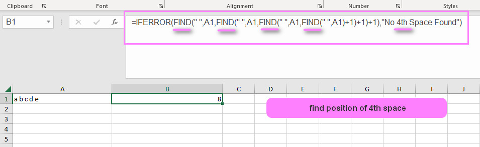
Let’s break down the formula step by step:
- “FIND(” “,A1,FIND(” “,A1,FIND(” “,A1,FIND(” “,A1)+1)+1)+1)” – This part of the formula searches for the fourth space character in the text string by nesting multiple FIND functions. Starting from the first space character, it looks for the next space character after every occurrence to reach the fourth space character.
- “IFERROR” – This function is used to handle error values in case the nth space character is not found in the text string.
- “No 4th Space Found” – This is the message that will display if the nth space character is not found.
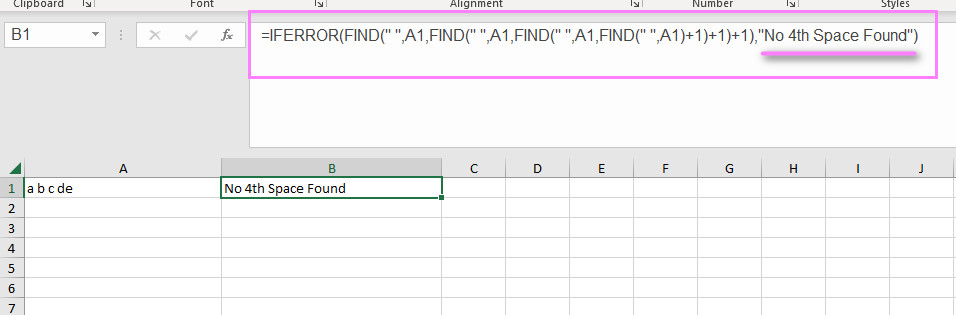
By using this formula, you can easily find the position of the nth space character in an Excel string.
Use the Trim formula to remove extra spaces
When working with text data in Excel, it is common to encounter extra spaces that can cause issues when analyzing or manipulating your data. The TRIM formula is a useful tool for removing these extra spaces.
The TRIM formula removes all leading and trailing spaces from a given text string, as well as any extra spaces between words. This helps to standardize your data and make it easier to work with.
Here’s how to use the TRIM formula:
- Select the cell(s) containing the text string(s) you want to trim.
- In the formula bar, type “=TRIM(” and then select the cell containing the text string, or manually enter the text string in quotation marks.
- Close the formula by typing “)” and hit enter.
For example, let’s say you have a list of names in column A, but some of the names contain extra spaces:
| Column A |
|---|
| John Smith |
| Jane Doe |
| Bob |
To remove the extra spaces, you can use the TRIM formula in column B like this:
- In cell B1, enter the formula “=TRIM(A1)”.
- Copy the formula down to the remaining cells in column B.
This will result in a trimmed version of your original data:
| Column A | Column B |
|---|---|
| John Smith | John Smith |
| Jane Doe | Jane Doe |
| Bob | Bob |
As you can see, the TRIM formula has removed the extra spaces from each name in column A, making the data more consistent and easier to work with.

In summary, the TRIM formula is a simple but powerful tool for cleaning up text data in Excel by removing extra spaces. It can save you time and prevent errors in your analysis by standardizing your data.
Using Find & Replace to remove extra spaces between words
When working with text data in Excel, sometimes there can be multiple spaces between words that make it difficult to analyze or manipulate the data. The Find & Replace feature in Excel provides an easy way to quickly remove all instances of extra spaces.
Here’s how to use Find & Replace to remove extra spaces:
- Select the range of cells containing the text strings you want to modify.
- Press Ctrl + H on your keyboard to open the Find & Replace dialog box.
- In the “Find what” field, enter two spaces by pressing the spacebar twice (or copy and paste a double space).
- In the “Replace with” field, enter a single space.
- Click the “Replace All” button.
For example, let’s say you have a list of addresses in column A, but some of the addresses contain extra spaces between words:
| Column A |
|---|
| 123 Main Street Anytown, USA 12345 |
| 456 Second Avenue Othertown, USA |
| 789 Third Street Somewhere, USA |
To remove the extra spaces, you can use Find & Replace like this:
- Select the range of cells containing the addresses (in this case, cells A1:A3).
- Press Ctrl + H to open the Find & Replace dialog box.
- In the “Find what” field, enter two spaces (press the spacebar twice).
- In the “Replace with” field, enter one space.
- Click the “Replace All” button.
This will result in a modified version of your original data:
| Column A |
|---|
| 123 Main Street Anytown, USA 12345 |
| 456 Second Avenue Othertown, USA |
| 789 Third Street Somewhere, USA |
As you can see, the extra spaces between words have been removed using Find & Replace.
Find space from right in Excel cell
In Excel, you can use the RIGHT function in combination with the LEN function to find the position of the last space in a cell from the right. Here are the steps to do so:
- Select the cell in which you want to find the last space from the right.
- Enter the following formula into the formula bar:
=LEN(A1)-FIND(" ",REVERSE(A1))Note that “A1” should be replaced with the cell reference of the cell you selected in step 1. - Press Enter, and the result will be displayed in the cell.
Let’s break down this formula:
LEN(A1)returns the length of the text in the cell.REVERSE(A1)reverses the order of the characters in the cell.FIND(" ", REVERSE(A1))finds the position of the first space in the reversed text.LEN(A1) - FIND(" ", REVERSE(A1))subtracts the position of the first space in the reversed text from the total length of the text, giving us the position of the last space in the original text from the right.
Finding the cell that contains just a space in Excel
Certainly! In Excel, you can use the TRIM function in combination with the LEN function to find cells that contain just a space. Here are the steps to do so:
- Select the range of cells in which you want to find cells that contain just a space.
- Enter the following formula into the formula bar:
=IF(LEN(TRIM(A1))=0,"Contains Just Space","Does Not Contain Just Space")Note that “A1” should be replaced with the first cell reference in the range you selected in step 1. - Press Enter, and the result will be displayed in the first cell of the range.
- Copy the formula down to the rest of the cells in the range.
Let’s break down this formula:
TRIM(A1)removes any leading or trailing spaces from the text in the cell.LEN(TRIM(A1))returns the length of the trimmed text.- If the length of the trimmed text is equal to 0, then the cell contains just a space. Otherwise, it does not.
The formula will return “Contains Just Space” for cells that contain just a space, and “Does Not Contain Just Space” for cells that contain any other text or characters.
How to Find and Replace Space in Excel
Here’s a step-by-step guide on how to find and replace space in Excel:
- Select the range of cells where you want to find and replace spaces. You can select a single cell, multiple cells, or an entire column or row.
- Press “Ctrl+H” on your keyboard to open the Find and Replace dialog box.
- In the “Find What” field, type a single space (press the spacebar once).
- Leave the “Replace With” field blank if you simply want to remove the spaces. If you want to replace the spaces with another character or text string, enter it in the “Replace With” field.
- Click on “Options” to see more options for finding and replacing spaces. For example, you can choose to match entire cells, match case, or search for specific formats.
- Click on “Find Next” to find the first occurrence of a space in the selected range. If you want to replace the space with the “Replace With” text, click on “Replace”. To replace all occurrences of the space in the selected range, click on “Replace All”.
- Repeat steps 6 and 7 until you have found and replaced all the spaces in the selected range.
Alternatively, you can use formulas or functions to find and replace spaces in Excel. For example, you can use the SUBSTITUTE function to replace spaces with another character or text string. Or you can use the TRIM function to remove extra spaces from a text string.
