The HLOOKUP function is one of the Lookup & reference functions of Excel.
It looks for a value in the top row of a table or array of values and returns the value in the same column from a row you specify.
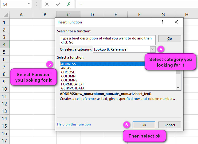
We can find this function in Lookup & reference of insert function Tab.
How to use HLOOKUP function in excel
- Click on empty cell (like F5).

2. Click on fx icon (or press shift+F3).

3. In insert function tab you will see all functions.

4. Select Lookup & reference category.
5. Select HLOOKUP function.
6. Then select ok.
7. In function arguments Tab, you will see HLOOKUP function.
8. Lookup_value is the value to be found in the first row of the table and can be a value, a reference, or a text string.
9. Table_array is a table of text, numbers, or logical values in which data is looked up. Table_array can be a reference to a range or a range name.
10. Row_index_num is the row number in table_array from which the matching value should be returned.The first row of values in the table is row 1.
11. Range_lookup is a logical value: to find the closest match in the top row (sorted in ascending order) = TRUE or omitted; find an exact match = FALSE.
12. You will see the result in formula result section
Examples of HLOOKUP function in excel
Here are examples of HLOOKUP in Excel:
1. Retrieving a single value from a table:=HLOOKUP("Product A",$A$2:$D$10,3,FALSE)
2. Retrieving the closest match to a lookup value:=HLOOKUP(lookup_value,table_array,row_index_num,TRUE)
3. Returning a specific cell in a row:=HLOOKUP("Product A",$A$2:$E$10,3,TRUE)
4. Finding the maximum value in a row:=HLOOKUP(MAX($B$1:$F$1),$A$1:$F$10,2,FALSE)
5. Filtering a dataset by specific criteria:=HLOOKUP("Product A",$A$2:$E$10,MATCH("Sales",$A$1:$E$1,0)+1,FALSE)
6. Identifying the row number of a value:=MATCH("Product A",$A$1:$A$10,0)
7. Finding the sum of a row:=SUM(HLOOKUP("Sales",$A$1:$F$10,MATCH("Product A",$A$1:$A$10,0),FALSE))
8. Returning the top N values in a row:=LARGE(HLOOKUP("Product A",$A$1:$F$10,ROW($A$1:$A$5),FALSE),1)
9. Identifying the column number of a value:=MATCH("Sales",$A$1:$F$1,0)
10. Using nested functions to perform multiple calculations:=IF(HLOOKUP("Product A",$A$1:$F$10,ROW($A$1:$A$10),FALSE)<100,"Low","High")
Syntax of HLOOKUP function in excel
The HLOOKUP function in Excel is used to search for a specific value in the top row of a table and return the corresponding value from a specified row.
The syntax for the HLOOKUP function is as follows:
=HLOOKUP(lookup_value, table_array, row_index_num, [range_lookup]).
HLOOKUP arguments:
– lookup_value:
This is the value that you want to search for in the top row of the table.
– table_array:
This is the range of cells that contains the table data. It must include the top row that contains the lookup value.
– row_index_num:
This is the row number in the table from which you want to return a value.
For example, if you want to return a value from the second row of the table, this argument would be 2.
– range_lookup:
This is an optional argument that specifies whether you want an exact match or an approximate match.
If you set this argument to TRUE or omit it, Excel will find the closest match to the lookup value.
If you set it to FALSE, Excel will only return an exact match.
For example, suppose you have a table of sales data with product names in the top row and sales figures for each month in subsequent rows.
If you want to find the sales figure for a particular product in a specific month, you could use the HLOOKUP function as follows:
=HLOOKUP("Product A", A1:F10, 3, FALSE).
In this example, “Product A” is the lookup value, A1:F10 is the range of cells containing the table data, 3 is the row index number (corresponding to the third row of the table, which contains sales data for January), and FALSE specifies that an exact match is required.
The function would return the sales figure for Product A in January.
Search for data in multiple rows with HLOOKUP function in excel
HLOOKUP is designed to search for data in a single row and return a value from a specified row.
If you need to search for data in multiple rows, you may need to use a combination of functions such as INDEX and MATCH or VLOOKUP.
Errors in HLOOKUP function in excel
several errors can occur when using this function, which can result in incorrect or unexpected results.
#N/A error:
This error occurs when the lookup value is not found in the table array. HLOOKUP returns #N/A if it cannot find a match.
To fix this error, users should check that the lookup value is spelled correctly and ensure that it exists in the table array.
#REF! error:
This error occurs when the column index number is greater than the number of columns in the table array. HLOOKUP returns #REF! if the column index number is out of range.
To fix this error, users should check that the column index number is within the range of the table array.
#VALUE! error:
This error occurs when the lookup value or the table array contains text instead of numbers. HLOOKUP returns #VALUE! if it cannot perform the lookup due to invalid data types.
To fix this error, users should ensure that the lookup value and table array contain only numeric values.
#NAME? error:
This error occurs when the function name is misspelled or not recognized by Excel. HLOOKUP returns #NAME? if there is a syntax error in the formula.
To fix this error, users should check that the function name is spelled correctly and ensure that it is recognized by Excel.
#NUM! error:
This error occurs when the range_lookup argument is not specified correctly. HLOOKUP returns #NUM! if the range_lookup argument is not a valid logical value (TRUE or FALSE).
To fix this error, users should ensure that the range_lookup argument is set to either TRUE or FALSE.
Search for values horizontally across rows with HLOOKUP
the HLOOKUP function in Excel can search for values horizontally across rows.
Here are examples to illustrate how the function works:
1. Suppose you have a table with sales information for different regions in columns A through E, and you want to retrieve the sales data for the West region.
You can use the HLOOKUP function as follows:
=HLOOKUP("West", A1:E4, 3, FALSE).
This will search for the value “West” in the first row of the table (A1:E1), and return the sales data for the West region in row 3 (A3:E3).
2. If you have a table with student grades for different subjects in rows 1 through 4, and you want to retrieve the grade for a particular student and subject,
you can use the HLOOKUP function.For example,
=HLOOKUP("Math", A1:E4, 2, FALSE).
will search for the value “Math” in row 1 (A1:E1), and return the grade for the student in row 2 (A2:E2).
3. Suppose you have a table with financial data for different quarters in columns A through D, and you want to retrieve the data for the second quarter.
You can use the HLOOKUP function as follows:
=HLOOKUP("Q2", A1:D4, 3, FALSE).
This will search for the value “Q2” in the first row of the table (A1:D1), and return the financial data for the second quarter in row 3 (A3:D3).
4. If you have a table with employee information, and you want to retrieve the salary for a particular employee, you can use the HLOOKUP function. For example,
=HLOOKUP("John Smith", A1:G4, 2, FALSE).
will search for the value “John Smith” in row 1 (A1:G1), and return the salary data for that employee in row 2 (A2:G2).
5. Suppose you have a table with product information in columns A through D, and you want to retrieve the price of a particular product.
You can use the HLOOKUP function as follows:
=HLOOKUP(“Product A”, A1:D4, 2, FALSE).
This will search for the value “Product A” in the first row of the table (A1:D1), and return the price data for that product in row 2 (A2:D2).
Lookup value is not found in the table array in HLOOKUP function
Here are examples that explain what happens if the lookup value is not found in the table array in HLOOKUP:
1. If the lookup value is numerical and not found in the first row of the table array, HLOOKUP will return the #N/A error.
2. If the lookup value is a text string and not found in the first row of the table array, HLOOKUP will also return the #N/A error.
3. If the lookup value is found in the first row of the table array but not in the specified column, HLOOKUP will return the value from the row that matches the lookup value but in a different column.
4. If the table array has only one row and the lookup value is not found, HLOOKUP will also return the #N/A error.
5. If the table array has multiple rows but none of the values in the first row match the lookup value, HLOOKUP will again return the #N/A error.
Use wildcards or regular expressions with HLOOKUP
Unfortunately, it is not possible to use wildcards or regular expressions with HLOOKUP function directly.
HLOOKUP is a function in Microsoft Excel that allows you to search for a value in the first row of a table or range, and then return a corresponding value in the same column from a specified row.
It only supports exact match or approximate match (using a range of values).
However, there are workarounds that you can use to achieve similar results.
One way is to use a combination of other functions like INDEX, MATCH, and LEFT to extract the desired values from the HLOOKUP range.
For example, you can use the LEFT function to extract a specific number of characters from the lookup value or the HLOOKUP range to match with the lookup value.
Another way is to use the VLOOKUP function instead of HLOOKUP and combine it with the ‘*’ or ‘?’ wildcards within your lookup value to perform a partial match.
The ‘*’ wildcard stands for any number of characters, while the ‘?’ wildcard stands for a single character.
For example, if you are looking for a value that starts with ‘ABC’, you can use the formula =VLOOKUP("ABC*", table, column, FALSE).
Keep in mind that both of these workarounds have their limitations and may not work in all situations.
It is always recommended to test your formulas thoroughly and consider the potential risks and limitations before relying on them.
Return multiple values with HLOOKUP function in excel
Unfortunately, HLOOKUP function in Microsoft Excel only allows you to return a single value.
It is designed to search for a value in the first row of a table, and then return a corresponding value in the same column based on a specified row index.
While it is not possible to use HLOOKUP to return multiple values, there are a few workarounds that you can use to get the desired result.
One commonly used method is to combine the INDEX and MATCH functions with HLOOKUP to create an array formula.
This allows you to return multiple values that match specific criteria.
Here are the steps to follow:
1. Select the cells where you want to display the results.
2. Enter the following formula in the first cell:
=IFERROR(INDEX($B$2:$E$5, MATCH($A$8, $A$2:$A$5, 0),0), "Not found").
In this formula,
$B$2:$E$5 refers to the range of cells where your table is located,
$A$8 refers to the value you are searching for, and
$A$2:$A$5 refers to the column where you want to search for the value.
3. Press CTRL+SHIFT+ENTER to convert the formula to an array formula.
This allows Excel to return an array of values instead of a single value.
4. Copy the formula to the remaining cells where you want to display the results.
Here’s a sample table to illustrate the formula:
| Name | Apple | Banana | Cherry | Date |
|——|——-|——–|——–|———-|
| Bob | 10 | 20 | 30 | 1/1/2023 |
| Jane | 15 | 25 | 35 | 1/2/2023 |
| John | 20 | 30 | 40 | 1/3/2023 |
| Sue | 25 | 35 | 45 | 1/4/2023 |
Suppose you want to search for the values associated with the name “Jane”.
You can use the array formula above to return all the values associated with that name across the row.
Another approach is to use the FILTER function in Excel which can be used to filter a table based on a specific condition.
Here are the steps:
1. Select the cells where you want to display the results.
2. Enter the following formula in the first cell:
=FILTER($B$2:$E$5, $A$2:$A$5="Jane")
In this formula, $B$2:$E$5 refers to the range of cells where your table is located, and $A$2:$A$5 refers to the column where you want to search for the value.
3. Press ENTER to display the result.
Use named ranges with HLOOKUP function in excel
The HLOOKUP function is a powerful tool in Excel that allows you to search for a value in the first row of a table and then return a value in the same column of a specified row number.
Using named ranges in your HLOOKUP formula can make your spreadsheets more readable and easier to maintain, especially if you’re working with large datasets.
Here’s an example of how to use HLOOKUP with named ranges in Excel:
1. First, select the range of cells you want to name.
Let’s say you have a table of sales data that spans from A1 to D10.
To name this range, click on the cell in the upper left corner (A1) and drag your mouse down to the bottom right corner (D10) to select the entire range.
Then, go to the “Formulas” tab in the ribbon and click “Define Name” in the “Defined Names” group.
Give your range a clear and concise name, such as “SalesData”, and click “OK”.
2. Now that you’ve named your range, you can use the HLOOKUP function to search for a value in the first row of the table and then return a corresponding value in a specified row number.
Let’s say you want to find the sales figures for a particular product in the month of March.
You can use the following formula:
=HLOOKUP("March", SalesData, 5, FALSE)
Here, “March” is the value you want to search for in the first row,
“SalesData” is the named range you defined earlier,
“5” is the row number you want to return sales figures for (assuming the table headers take up the first 4 rows), and
“FALSE” tells Excel to look for an exact match for the search term.
3. When you enter this formula in a cell, Excel will search the first row of the named range (SalesData) for the value “March” and then return the corresponding value from the 5th row of the table, which contains the sales data for each product.
Speed up your HLOOKUP function in excel
HLOOKUP function in Excel is used to search for a specific value in the first row of a table and return the corresponding value in a specified row.
However, HLOOKUP can become slow, especially when used with large data sets or complex formulas.
Here are some ways to speed up your HLOOKUP formulas:
1. Simplify your data:
Complex data sets and formulae can slow down HLOOKUP.
Simplify your data by removing unnecessary formulas, rows or columns, and use tables instead of ranges.
Example:
Instead of referencing a range of cells in your formula, use a table.
Tables have a clear structure and allow you to reference columns by name rather than by cell references, which makes your formulas easier to read and understand.
2. Use INDEX MATCH instead of HLOOKUP:
INDEX MATCH is a more flexible and efficient alternative to HLOOKUP.
It allows you to search horizontally or vertically and lookup values from any column, not just the leftmost column.
Example:
Instead of using HLOOKUP, you can use INDEX MATCH like this:
=INDEX(A1:C4,MATCH("Value1",B1:B4,0),3)
This formula searches for “Value1” in column B and returns the corresponding value in column C.
3. Use the approximate match feature:
When you don’t need an exact match, you can use the approximate match feature of HLOOKUP to speed up your formula.
Approximate match returns the closest match to the lookup value, rather than an exact match.
Example:
Instead of using an exact match HLOOKUP like this:
=HLOOKUP("lookup_value",A1:C4,2,FALSE)
You can achieve faster results by using an approximate match like this:
=HLOOKUP("lookup_value",A1:C4,2,TRUE)
In conclusion, speeding up HLOOKUP formulas in Excel can be achieved by simplifying your data, using INDEX MATCH instead of HLOOKUP, and using the approximate match feature when appropriate.
Conditional formatting in HLOOKUP function in excel
HLOOKUP is a function in Excel that looks for a value in the top row of a table and returns a corresponding value in the same column from a row you specify.
Conditional formatting, on the other hand, is a feature that allows you to format cells based on predefined criteria.
To use HLOOKUP with conditional formatting, you can use the following steps:
1. Identify the cell range that you want to apply the formatting to.
2. Go to the “Conditional Formatting” menu and select “New Rule.”
3. In the “New Formatting Rule” window, select “Use a formula to determine which cells to format.”
4. Enter the HLOOKUP formula in the formula box.
For example, let’s say you have a table with product names in row 1, and you want to format cells based on the value in row 2.
You can enter the following formula:
=HLOOKUP(“Apples”,$A$1:$E$2,2,FALSE)
where “Apples” is the value you want to look up and
$A$1:$E$2 is the range containing the lookup value and the values to return.
The 2 specifies the row number you want to return values from, and
FALSE means you want an exact match for the lookup value.
5. Select the formatting options you want to apply to the cells that meet the criteria.
6. Click “OK” to apply the formatting.
For example, let’s say you have a table that lists the sales of various products, and you want to highlight cells where the sales of “Apples” are greater than $1000.
You can use the following steps:
1. Select the cell range that contains the sales data for the products, including the product names in the top row.
2. Go to “Conditional Formatting” and select “New Rule.”
3. In the “New Formatting Rule” window, select “Use a formula to determine which cells to format.”
4. Enter the HLOOKUP formula in the formula box:
=HLOOKUP("Apples",$A$1:$E$2,2,FALSE)>1000
5. Select the formatting options you want to apply to the cells that meet the criteria, such as a fill color or font color.
6. Click “OK” to apply the formatting.
This will highlight all cells in the row for “Apples” where the sales value is greater than $1000.
Difference between HLOOKUP and VLOOKUP
VLOOKUP and HLOOKUP are two popular lookup functions in Microsoft Excel, used to search for specific data within a range or table.
The main differences between the two are as follows:
VLOOKUP (Vertical Lookup)
– VLOOKUP searches vertically (in a column) for a specific value in the leftmost column of the table.
– This function returns a value from the same row as the lookup value, but from a specified column in the table.
– It is useful for looking up information in a database-like table where a unique identifier (such as customer ID, product code, or employee number) is in the first (leftmost) column.
HLOOKUP (Horizontal Lookup)
– HLOOKUP searches horizontally (in a row) for a specific value in the top row of the table.
– This function returns a value from the same column as the lookup value, but from a specified row in the table.
– It is useful for looking up information in a table where the first row contains the field names (such as product names, months, or department names), and the rest of the table contains data.
In summary, VLOOKUP is used to search for data in a table by looking up a value in the leftmost column of the table and returning a corresponding value from a specified column.
HLOOKUP is used to search for data in a table by looking up a value in the top row of the table and returning a corresponding value from a specified row.
Both functions can be very useful for quickly finding and analyzing data within a large Excel spreadsheet.


