What is ADDRESS Function in Excel?
The ADDRESS function is one of the Lookup & reference functions of Excel.
It Creates a cell reference as text, given specified row and column numbers.
We can find this function in Lookup & reference of insert function Tab.
How to use ADDRESS function in excel
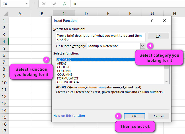
- Click on an empty cell (like F5 ).

2. Click on the fx icon (or press shift+F3).

3. In the insert function tab you will see all functions.

4. Select Lookup & reference category.
5. Select ADDRESS function.
6. Then select ok.
7. In the function arguments Tab, you will see ADDRESS function.
8. Row num is the row number to use in the cell reference. For example,Row number = 1 for row 1.
9. Column_num section is the column number to use in the cell reference. For example, Column number = 4 for column D.
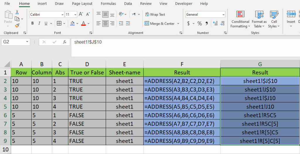
10. Abs num specifies the reference type: absolute = 1; absolute row/relative column = 2; relative row/absolute column = 3; relative = 4.
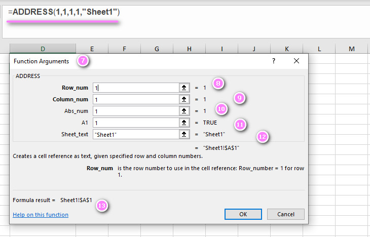
11. A1 is a logical value that specifies the reference style: A1 style = 1 or TRUE; R1 C1 style = 0 or FALSE.
12. Sheet text is text specifying the name of the worksheet to be used as the external reference.
13. You will see the result in formula result section.
Examples of ADDRESS function in excel
- =ADDRESS(2,3) – returns the cell address for row 2 and column 3 (i.e. “C2”)
- =ADDRESS(5,7,2) – returns the absolute cell reference (with dollar signs) for row 5 and column 7 (i.e. “$G$5”)
- =ADDRESS(1,1,4) – returns the cell reference using R1C1-style notation for row 1 and column 1 (i.e. “R1C1”)
- =ADDRESS(3,2,4,TRUE,”Sheet2″) – returns the cell reference using R1C1-style notation for row 3 and column 2 on Sheet2 (i.e. “Sheet2!R3C2”)
- =ADDRESS(ROW(A1),COLUMN(A1)) – returns the address of the cell containing A1 (i.e. “$A$1”)
- =ADDRESS(3,2)+2 – returns the address of the cell two columns to the right of row 3, column 2 (i.e. “D3”)
- =ADDRESS(3,2,,,”Sheet2″) – returns the address of the cell in row 3, column 2 on Sheet2 (i.e. “Sheet2!B3”)
- =ADDRESS(ROW(),COLUMN()) – returns the address of the current cell
- =ADDRESS(3,COLUMN()+1) – returns the address of the cell one column to the right of column C and in row 3 (i.e. “D3”)
- =ADDRESS(ROW(A1)+2,COLUMN(A1)-1) – returns the cell address two rows below and one column to the left of cell A1 (i.e. “A3”)
Excel’s ADDRESS Function: Understanding Its Purpose and Usage
The ADDRESS function in Excel is used to return a cell reference address as a text string, based on a given row and column number. This function can be very useful when constructing other formulas and functions that require a cell reference.
Learning the Arguments of Excel’s ADDRESS Function
The ADDRESS function requires three arguments:
- Row_num: This argument specifies the row number of the cell reference that you want to retrieve.
- Column_num: This argument specifies the column number of the cell reference that you want to retrieve.
- [Abs_num]: This argument is optional and specifies the type of reference that you want to return: 1 = absolute (default), 2 = relative, 3 = mixed.
How to Use Excel’s ADDRESS Function to Retrieve a Cell Address
To use the ADDRESS function, simply enter it into a cell and specify the required arguments within the parentheses. For example, to retrieve the address for cell D4, use the formula:
=ADDRESS(4,4)
This will return the text string “$D$4”, which represents the absolute cell reference for cell D4.
Using Excel’s ADDRESS Function for Absolute References
You can also use the optional Abs_num argument to change the reference type returned by the ADDRESS function. For example, to retrieve a mixed cell reference for row 4 and column 4, with an absolute row reference, use the formula:
=ADDRESS(4,4,3)
This will return the text string “$D4”, which represents the mixed cell reference for column D and row 4, with an absolute row reference.
In conclusion, the ADDRESS function is a powerful tool in Excel that can help you construct more complex formulas and functions that require cell references. By understanding its arguments and usage, you can use this function to streamline your workflow and improve your productivity.
Employing Excel’s ADDRESS Function for Relative References
In addition to using the ADDRESS function to retrieve absolute or mixed cell references, you can also use it to return a relative reference. To do this, simply omit the optional Abs_num argument from the formula. For example, to retrieve the relative reference for the cell one column to the right and one row down from the current cell, use the formula:
=ADDRESS(ROW()+1,COLUMN()+1)
This will return the text string “B2” if entered into cell A1.
Setting Up Mixed References with Excel’s ADDRESS Function
Excel’s ADDRESS function can also be used to create mixed references – where one part of the cell reference is absolute and the other part is relative. To set up a mixed reference, use the optional Abs_num argument to specify which part of the reference should be absolute. For example, to create a reference that is fixed to column B but changes according to the current row number, use the formula:
=ADDRESS(ROW(),2,4)
This will return a text string like “$B1” in cell A1, which represents the mixed reference for column B and the current row.
Creating Dollar Sign References with Excel’s ADDRESS Function
Dollar sign references are another type of absolute reference in Excel. They are commonly used in formulas and functions to fix a specific cell reference in place. To create a dollar sign reference with the ADDRESS function, use the optional Abs_num argument and set it to 1. For example, to retrieve an absolute reference for cell C5, use the formula:
=ADDRESS(5,3,1)
This will return the text string “$C$5”.
Excel’s ADDRESS Function: Retrieving a Range of Cells
Finally, you can use the ADDRESS function to retrieve a range of cells by combining it with the INDIRECT function. For example, to retrieve the range of cells from A1 to B2, use the formula:
=INDIRECT(ADDRESS(1,1)&”:”&ADDRESS(2,2))
This will return the range A1:B2.
In conclusion, the ADDRESS function in Excel is a versatile tool that can help you create a range of cell references, from relative to absolute to mixed. By understanding its usage and combining it with other functions like INDIRECT, you can unlock new capabilities and improve your productivity in Excel.
Excel’s ADDRESS Function in R1C1-Style Notation
Excel allows users to work with cell references in two different styles – the A1 notation and the R1C1 notation. The A1 notation (the default style) refers to cells using letters for columns and numbers for rows, while the R1C1 notation refers to cells using numbers for both rows and columns, where “R” stands for row and “C” stands for column.
To use Excel’s ADDRESS function in R1C1-style notation, simply set the optional Row_abs and Column_abs arguments to 0. For example, to retrieve the R1C1-style reference for cell two rows down and three cells to the right of the current cell, use the formula:
=ADDRESS(ROW()+2,COLUMN()+3,4,1,0)
This will return the text string “R[2]C[3]” if entered into cell A1.
Referencing Cells on a Specific Worksheet with Excel’s ADDRESS Function
If your workbook contains multiple worksheets, you can use Excel’s ADDRESS function to reference cells on a specific worksheet by including the sheet name as an argument. For example, to retrieve the address for cell B1 on a worksheet named “Sheet2”, use the formula:
=ADDRESS(1,2,4,1,”Sheet2″)
This will return the text string “Sheet2!$B$1”.
Excel’s ADDRESS Function: Retrieving a Named Range
A named range is a group of cells that have been given a name to make them easier to work with in formulas and functions. To retrieve the address of a named range using Excel’s ADDRESS function, simply enter the name of the range as the first argument. For example, to retrieve the address for a named range called “SalesData”, use the formula:
=ADDRESS(“SalesData”)
This will return the text string “$A1:1:C$10”, which represents the address of the named range.
Using Row and Column Numbers with Excel’s ADDRESS Function
In addition to specifying the row and column numbers directly, you can also use cell references or formulas that return row and column numbers as arguments for Excel’s ADDRESS function. For example, to retrieve the address for a cell that is three columns to the right of the cell in column A and in the same row, use the formula:
=ADDRESS(ROW(),COLUMN(A:A)+3)
This will return the text string “$A$1” if entered into cell A1.
In conclusion, Excel’s ADDRESS function is a powerful tool that can help you work with cell references in a variety of ways, including R1C1-style notation, referencing cells on specific worksheets, retrieving named ranges, and using row and column numbers. By understanding its usage and capabilities, you can improve your productivity and streamline your workflow in Excel.
How to Find the Current Cell Address with Excel’s ADDRESS Function
Excel’s ADDRESS function can also be used to find the current cell address in a worksheet. To do this, simply omit the row_num and column_num arguments from the formula. The resulting text string will represent the address of the cell in which the formula is entered. For example, if you enter the formula:
=ADDRESS()
in cell A1, it will return the text string “$A$1”.
Creating Relative References with Excel’s ADDRESS Function
Excel’s ADDRESS function can be used to create relative cell references that change based on the position of the formula in the worksheet. To create a relative reference, simply omit the optional Abs_num argument from the formula. For example, to retrieve the relative reference one row below and one column to the right of the current cell, use the formula:
=ADDRESS(ROW()+1,COLUMN()+1)
This will return the text string “B2” if entered into cell A1.
Excel’s ADDRESS Function: Retrieving a Cell Address Relative to Another Cell
You can also use Excel’s ADDRESS function to retrieve a cell address relative to another cell in the worksheet. To do this, subtract the row number and column number of the reference cell from the row number and column number of the target cell, respectively. For example, to retrieve the address for a cell that is two rows down and three columns to the right of cell C3, use the formula:
=ADDRESS(ROW(C3)+2,COLUMN(C3)+3)
This will return the text string “F5”.
Excel’s ADDRESS Function: Complementing Other Functions
Excel’s ADDRESS function can complement other functions when working with cell references. For example, you can use it with the MATCH function to retrieve the address of a matched value in a range, or with the INDEX function to retrieve a specific cell within an array.
In conclusion, Excel’s ADDRESS function is a versatile tool that can help you work with cell references in a variety of ways, including finding the current cell address, creating relative references, retrieving cell addresses relative to other cells, and complementing other functions. By understanding its usage and capabilities, you can improve your productivity in Excel and streamline your workflow.
Dynamic Referencing Techniques with Excel’s ADDRESS Function
Excel’s ADDRESS function can be used to create dynamic referencing techniques that adjust automatically as the worksheet data changes. For example, you can use the ROWS and COLUMNS functions to create a reference that adjusts based on the size of a range. To retrieve the address of the last cell in a range, use the formula:
=ADDRESS(ROW(range)+ROWS(range)-1,COLUMN(range)+COLUMNS(range)-1)
This will return the address of the last cell in the range.
Customizing Your Reference Format with Excel’s ADDRESS Function
Excel’s ADDRESS function allows for customization of the reference format to fit specific needs. For example, you can use text strings to add labels or separators to the cell reference. To retrieve a custom cell reference that includes a label for the column and a separator between the row and column, use the formula:
=ADDRESS(2,3)&” (Total Sales)”
This will return the text string “C2 (Total Sales)”.
Finding the Last Cell in a Range with Excel’s ADDRESS Function
Excel’s ADDRESS function can also be used to find the address of the last cell in a range, regardless of its size. To do this, use the COUNTA function to count the number of non-empty cells in the range, then subtract one from the result to get the row number of the last cell. Use this value as the row_num argument in the ADDRESS function, and specify the last column in the range as the column_num argument. For example, to retrieve the address of the last cell in a range that starts at A1, use the formula:
=ADDRESS(COUNTA(A:A)-1,COLUMNS(range),4)
This will return the address of the last cell in the range.
Excel’s ADDRESS Function: Retrieving a Cell Based on a Logical Condition
Excel’s ADDRESS function can be used to retrieve a cell based on a logical condition using the INDEX function. For example, to retrieve the address of the first cell in a range that contains a specific value (e.g. “Apples”), use the formula:
=ADDRESS(MATCH(“Apples”,range,0),COLUMN(range))
This will return the address of the first cell in the range that contains “Apples”.
In conclusion, Excel’s ADDRESS function is a powerful tool that can help you create dynamic referencing techniques, customize reference formats, find the last cell in a range, and retrieve cells based on logical conditions. By understanding its usage and combining it with other functions like MATCH and INDEX, you can unlock new capabilities and improve your productivity in Excel.
ADDRESS related functions
- INDIRECT function
- ROW function


