What is CHOOSE function in Excel ?
The CHOOSE function is one of the Lookup & reference functions of Excel.
It Chooses a value or action to perform from a list of values, based on an index number.
We can find this function in Lookup & reference category of insert function Tab.
How to use CHOOSE function in excel
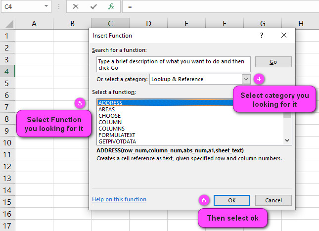
- Click on an empty cell (like F5 ).

2. Click on the fx icon (or press shift+F3).

3. In the insert function tab you will see all functions.

4. Select Lookup & reference category.
5. Select CHOOSE function.
6. Then select ok.
7. In the function arguments Tab, you will see CHOOSE function.
8. Index num section specifies which value argument is selected.
Index num must be between 1 and 254, or a formula or a reference to a number between 1 and 254.
9. Value1: value1,value2,… are 1 to 254 numbers, cell references, defined names, formulas, functions, or text arguments from which CHOOSE selects.
10. You will see the result in the formula result section

Examples of CHOOSE function in excel

Examples of CHOOSE function
- =CHOOSE(2,”Apple”,”Banana”,”Cherry”) – This formula returns “Banana” because it is the second item in the list.
- =CHOOSE(B2,”Small”,”Medium”,”Large”) – If cell B2 contains the value 3, this formula returns “Large”.
- =CHOOSE(A1,A2,A3,A4,A5) – This formula uses the value in cell A1 to choose one of the values in the range A2:A5.
- =CHOOSE(WEEKDAY(TODAY()),”Sunday”,”Monday”,”Tuesday”,”Wednesday”,”Thursday”,”Friday”,”Saturday”) – This formula returns the name of the current day of the week.
- =CHOOSE(RAND()*5+1,”Red”,”Green”,”Blue”,”Yellow”,”Purple”) – This formula chooses a random color from the list.
- =CHOOSE(MONTH(A1),”Winter”,”Winter”,”Spring”,”Spring”,”Spring”,”Summer”,”Summer”,”Summer”,”Fall”,”Fall”,”Fall”,”Winter”) – This formula returns the season based on the month in cell A1.
- =CHOOSE(IF(B2>50,2,1),”Low”,”High”) – If cell B2 contains a value greater than 50, this formula returns “High”, otherwise it returns “Low”.
- =CHOOSE(LEN(A1),A1&”s”,A1&”es”) – This formula adds “s” or “es” to the end of the text in cell A1, depending on its length.
- =CHOOSE(VLOOKUP(A1,B2:C10,2,FALSE),”Yes”,”No”) – This formula looks up the value in cell A1 in the range B2:C10 and returns “Yes” if the value is found in column 2, or “No” otherwise.
- =CHOOSE(DAY(A1),1,2,3,4,5,6,7,8,9,10,11,12,13,14,15,16,17,18,19,20,21,22,23,24,25,26,27,28,29,30,31) – This formula returns the day of the month as a number from 1 to 31.
Master Excel’s Choose Function: Understanding its Syntax
The CHOOSE function in Excel allows you to select a value from a list of values based on the index number. It has a simple syntax that involves specifying the index number and the list of values. For example, if you have a list of fruits such as apples, bananas, and cherries in cells A1:A3, you can use the CHOOSE function to select the fruit based on an index number entered by the user in cell B1. The formula would be “=CHOOSE(B1,A1:A3)”.
Choosing Values Made Easy: Excel’s Choose Function Explained
Excel’s CHOOSE function is a powerful tool that makes selecting values from a list easy. It allows you to set up a menu of options and quickly select the value you need. For example, imagine you have a spreadsheet with a list of products in column A and their corresponding prices in column B. You want to create a dropdown menu so that the user can choose a product and see its price. By using the CHOOSE function, you can easily create this functionality. The formula would be “=CHOOSE(A1,B1:B3)” where A1 contains the index number selected by the user.
Selecting Options with Ease: How to Use Excel’s Choose Function
Excel’s CHOOSE function is a versatile tool that can be used for a variety of tasks. One common use case is creating dynamic charts or graphs. For example, imagine you have a chart that shows the sales data for different regions over time. You want to give the user the ability to switch between different regions by selecting them from a dropdown menu. By using the CHOOSE function, you can achieve this functionality easily. The formula would be “=CHOOSE(A1,Region1!$B2:B10,Region2!B2:B10,,Region3!B2:B$10)” where A1 contains the index number selected by the user and Region1, Region2, and Region3 are different worksheets containing the sales data for those regions.
Choose Your Arguments Wisely: Maximize the Potential of Excel’s Choose Function
The CHOOSE function in Excel is a powerful tool that can save you time and improve the functionality of your spreadsheets. However, it’s important to choose your arguments carefully to maximize its potential. For example, if you’re using the CHOOSE function to create a dropdown menu, make sure to use named ranges instead of cell references to avoid errors when inserting or deleting rows. Additionally, be mindful of the maximum number of values that can be included in the CHOOSE function (255), and consider using alternative functions such as INDEX-MATCH for more complex tasks.
Efficiently Reference Cells: Using Cell References in Excel’s Choose Function
When using the CHOOSE function in Excel, it’s important to efficiently reference cells to avoid errors and make your formulas easier to read. One way to do this is by using cell references in your list of values instead of hardcoding them directly into the formula. For example, if you have a list of monthly sales data in cells A1:A12, you can reference this range in your CHOOSE function by entering “=CHOOSE(A13,A1:A12)” where A13 contains the index number selected by the user.
Turning Textual Data into Insights: Utilizing Excel’s Choose Function for Text Values
While the CHOOSE function in Excel is commonly used with numeric values, it can also be used with textual data to extract insights from large datasets. For example, imagine you have a spreadsheet containing customer feedback comments and you want to categorize them into positive, neutral, or negative. By using the CHOOSE function, you can create a formula that assigns each comment to a category based on specific keywords. The formula would be something like “=CHOOSE(SUM(IFERROR(SEARCH({“good”,”great”,”excellent”},A1),0)), “Negative”, “Neutral”, “Positive”)” where A1 contains the customer feedback comment.
Number Crunching Made Simple: Excel’s Choose Function for Numeric Values
The CHOOSE function in Excel is a powerful tool for number crunching tasks such as calculating averages, sums, or weighted values. For example, imagine you have a dataset containing test scores for different subjects and you want to calculate the overall score for each student based on their performance in each subject. By using the CHOOSE function, you can easily create a formula that takes into account the weights of each subject. The formula would be something like “=SUM(CHOOSE(A1,B1:D1)*{0.4,0.3,0.3})” where A1 contains the index number of the subject and B1:D1 contain the test scores for that subject.
Deep Dive into Excel Functions: Nesting Choose Function Inside Other Functions
The CHOOSE function in Excel can also be nested inside other functions to create more complex formulas. For example, imagine you have a dataset containing sales data for different products and regions, and you want to calculate the total revenue for each product. By using the CHOOSE function inside a SUMIF function, you can easily create a formula that calculates the total revenue based on the selected region. The formula would be something like “=SUMIF(A1:A100,CHOOSE(B1,”Product1″,”Product2″,”Product3″),C1:C100)” where A1:A100 contains the product names, B1 contains the index number of the selected product, and C1:C100 contains the corresponding revenue data.
#VALUE! Errors No More: Resolving Issues with Excel’s Choose Function
The CHOOSE function in Excel can sometimes produce #VALUE! errors if the index number entered by the user is not within the range of available options. To avoid this issue, you can use an IF statement to check if the index number is valid before using the CHOOSE function. For example, the formula could be “=IF(B1<=COUNT(A1:A3),CHOOSE(B1,A1:A3),”Index out of range”)” where B1 contains the index number selected by the user and A1:A3 contains the list of values.
Avoiding #REF! Errors: Best Practices for Excel’s Choose Function
Another common error when using the CHOOSE function in Excel is the #REF! error, which occurs when a cell reference in the list of values is deleted or moved. To avoid this issue, it’s best to use named ranges instead of cell references in your CHOOSE function. For example, imagine you have a named range called “Fruits” that contains the values “Apples”, “Bananas”, and “Cherries”. You can then use this named range in your CHOOSE function by entering “=CHOOSE(B1,Fruits)” where B1 contains the index number selected by the user.
Conditional Formatting Just Got Better: Using Excel’s Choose Function for Styling
The CHOOSE function in Excel can also be used with conditional formatting to style cells based on specific conditions. For example, imagine you have a dataset containing sales data for different regions, and you want to highlight the top-performing region for each product. By using the CHOOSE function inside a MAX function, you can easily create a formula that identifies the maximum value and applies conditional formatting to the corresponding cell. The formula would be something like “=MAX(CHOOSE(A1,B1:B10,C1:C10,D1:D10))” where A1 contains the index number of the selected product, and B1:B10, C1:C10, and D1:D10 contain the sales data for each region.
Validation Made Easy: Employing Excel’s Choose Function with Data Validation
The CHOOSE function in Excel can also be used with data validation to create dropdown menus that allow the user to select from a list of options. For example, imagine you have a dataset containing customer feedback scores, and you want to create a dropdown menu that allows the user to select from predefined options such as “Excellent”, “Good”, “Fair”, or “Poor”. By using the CHOOSE function inside a data validation rule, you can easily create this functionality. The formula would be something like “=CHOOSE(B1,”Poor”,”Fair”,”Good”,”Excellent”)” where B1 contains the index number selected by the user.
Excel at Array Formulas: Using the Choose Function for Advanced Calculations
The CHOOSE function in Excel can also be used with array formulas to perform advanced calculations. For example, imagine you have a dataset containing sales data for different products and regions, and you want to calculate the total revenue for each product based on the top-performing region. By using the CHOOSE function inside an array formula, you can easily create a formula that identifies the maximum sales data for each product and multiplies it by the corresponding price. The formula would be something like “{=MAX(CHOOSE(A1,B1:B10,C1:C10,D1:D10)*{100,200,300})}” where A1 contains the index number of the selected product, B1:B10, C1:C10, and D1:D10 contain the sales data for each region, and {100,200,300} contains the prices for each product.
Dynamic Drop-down Lists Made Simple: Utilizing Excel’s Choose Function
The CHOOSE function in Excel can also be used to create dynamic drop-down lists that automatically update based on the selected category. For example, imagine you have a dataset containing information about different cars such as their make, model, and year. You want to create a drop-down menu that allows the user to first select the make, and then only shows the models for that particular make. By using the CHOOSE function inside a data validation rule, you can easily create this functionality. The formula would be something like “=CHOOSE(B1,”Toyota”,”Honda”,”Ford”)” where B1 contains the index number of the selected make, and the list of values for each make is located in separate named ranges.
Advanced Lookup Techniques: Leveraging VLOOKUP or INDEX/MATCH with Excel’s Choose Function
The CHOOSE function in Excel can also be combined with other lookup functions such as VLOOKUP or INDEX/MATCH to perform advanced data lookups. For example, imagine you have a dataset containing customer information such as their name, address, and phone number, and you want to create a formula that retrieves their phone number based on their name and address. By using the CHOOSE function inside an INDEX/MATCH formula, you can easily create this functionality. The formula would be something like “=INDEX(C1:C100,MATCH(B1&” “&CHOOSE(A1,”Street”,”Avenue”,”Road”),A1:A100&B1:B100,0))” where A1 contains the index number of the selected address type, B1 contains the street address, C1:C100 contains the phone numbers, and A1:A100&B1:B100 contain the names and addresses.
Making Multiple Conditions Work: Excel’s Choose Function and IF Statements
The CHOOSE function in Excel can also be combined with IF statements to create formulas that take into account multiple conditions. For example, imagine you have a dataset containing sales data for different products and regions, and you want to calculate a bonus for each salesperson based on their performance in each region. By using the CHOOSE function inside an IF statement, you can create a formula that assigns different bonus amounts based on specific sales targets. The formula would be something like “=IF(B1>=100000,CHOOSE(C1,500,750,1000),IF(B1>=75000,CHOOSE(C1,250,375,500),IF(B1>=50000,CHOOSE(C1,100,150,200),0)))” where B1 contains the sales data for the region, C1 contains the index number of the selected product, and the CHOOSE function contains the corresponding bonus amount for each product.
Streamlining Data Analysis: Using Excel’s Choose Function with SUMIF or COUNTIF
The CHOOSE function in Excel can be used with the SUMIF or COUNTIF functions to streamline data analysis tasks. For example, imagine you have a dataset containing customer feedback scores for different products and you want to calculate the average score for each product category (e.g. electronics, clothing, beauty). By using the CHOOSE function inside a SUMIF formula, you can easily create a formula that calculates the total score based on the selected category. The formula would be something like “=SUMIF(A1:A100,CHOOSE(B1,”Electronics”,”Clothing”,”Beauty”),C1:C100)” where A1:A100 contains the product categories, B1 contains the index number of the selected category, and C1:C100 contains the corresponding scores.
PivotTable Power-Up: Excel’s Choose Function as a Calculated Field
The CHOOSE function in Excel can also be used as a calculated field in a PivotTable to perform advanced calculations. For example, imagine you have a PivotTable containing sales data for different regions and products, and you want to calculate the total revenue for each product category (e.g. electronics, clothing, beauty) based on the selected region. By using the CHOOSE function inside a calculated field, you can easily create a formula that identifies the selected region and multiplies it by the corresponding price. The formula would be something like “=CHOOSE(B1,”Electronics”,”Clothing”,”Beauty”)*C1″ where B1 contains the index number of the selected category, and C1 contains the corresponding price.
Limits of Excel’s Choose Function: Cannot Select Ranges of Cells
While the CHOOSE function in Excel is a powerful tool for selecting values from a list, it has some limitations. One limitation is that it cannot be used to select ranges of cells. For example, imagine you have a dataset containing sales data for different products and regions, and you want to calculate the total revenue for each product by summing the corresponding sales data for each region. While you could use the CHOOSE function to select the sales data for each region, you cannot use it to select a range of cells. Instead, you would need to use another function such as SUM or SUMIF to perform this calculation.
Customizing Calculations with User Input: Excel’s Choose Function at Your Service
The CHOOSE function in Excel can also be used to customize calculations based on user input. For example, imagine you have a dataset containing sales data for different products and regions, and you want to create a formula that calculates the revenue based on the selected sales tax rate. By using the CHOOSE function inside a simple multiplication formula, you can easily create a formula that takes into account the selected tax rate. The formula would be something like “=B1*CHOOSE(A1,0.05,0.06,0.07)” where A1 contains the index number of the selected tax rate, B1 contains the revenue data, and the CHOOSE function contains the corresponding tax rate for each option.
CHOOSE related functions
- IF function
- MATCH function
- SWITCH function
- VLOOKUP function
