What is COLUMN function in Excel?
The COLUMN function is one of the Lookup & reference functions of Excel.
It Returns the column number of a reference.
We can find this function in Lookup & reference category of the insert function Tab.
How to use COLUMN function in excel
- Click on an empty cell (like F5 ).

2. Click on the fx icon (or press shift+F3).

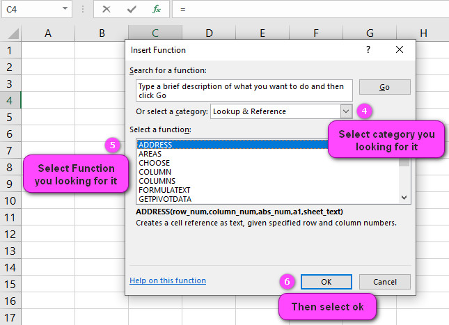
3. In the insert function tab you will see all functions.

4. Select Lookup & reference category.
5. Select COLUMN function.
6. Then select ok.
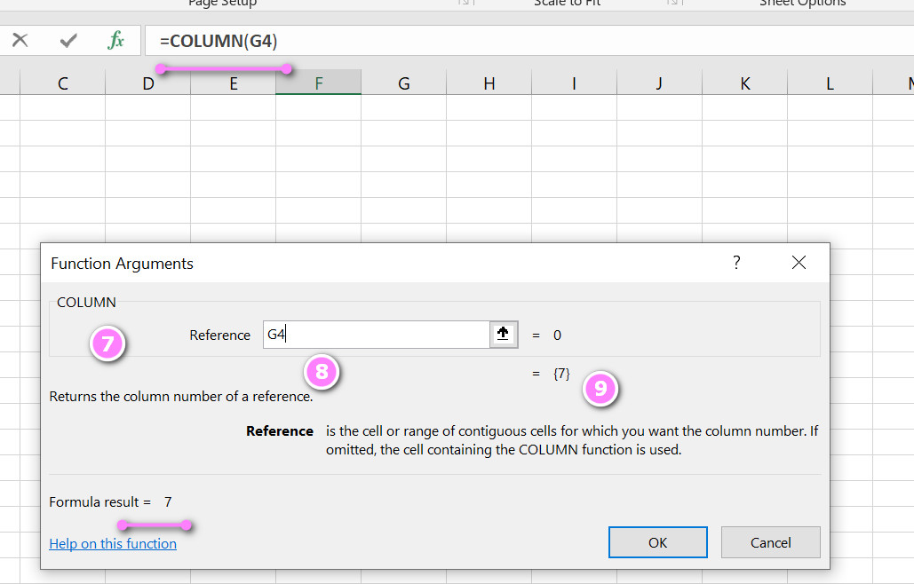
7. In the function arguments Tab, you will see the COLUMN function.
8. Reference is the cell or range of contiguous cells for which you want the column number.
9. For example If you click on G4, see result= 7.
10. If you click on A4 , see result =1.
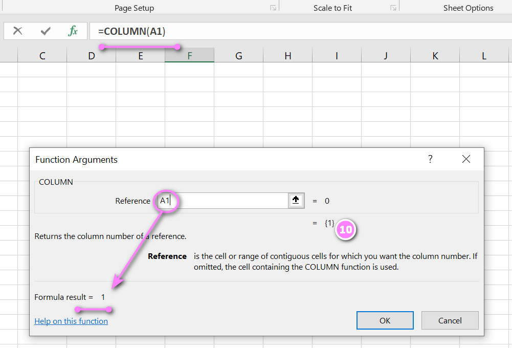
11. You will see the result in the formula result section.
Examples of COLUMN function in excel

Unleash the Power of Column Functions in Excel!
Excel provides a wide range of powerful column functions that can help you manipulate and analyze your data quickly and easily. One popular function is SUMIF, which allows you to sum up values in a range based on a specified condition. For example, if you have a sales report with columns for product names, prices, and quantities sold, you could use the SUMIF function to calculate the total revenue generated by a specific product.
Inserting a New Column: A Beginner’s Guide
Inserting a new column in Excel is a simple process that can be done in just a few clicks. To insert a new column, simply right-click on the column next to where you want to insert the new column and select “Insert” from the drop-down menu. You can also go to the “Home” tab on the ribbon and click on the “Insert” button. A new column will appear to the left of the selected column.
Row vs. Column in Excel: Understanding the Basics
Rows and columns are the two fundamental components of an Excel spreadsheet. Rows run horizontally across the sheet, while columns run vertically. Rows are typically used to organize and display data, while columns are used to define attributes or characteristics of the data. For example, in a table of customer information, rows might represent individual customers while columns might include fields for name, address, phone number, etc.
Deleting Columns Made Easy with Excel
Deleting a column in Excel is a straightforward process that requires only a few clicks. Simply select the column you want to delete by clicking on its header, then right-click and choose “Delete” from the drop-down menu. Alternatively, you can go to the “Home” tab on the ribbon and click on the “Delete” button. Be sure to double-check that you have selected the correct column before deleting it, as this action cannot be undone.
Hiding Columns in Excel: Tips and Tricks
Hiding columns in Excel is a great way to declutter your worksheet and make it easier to read. To hide a column, simply right-click on the column header and select “Hide” from the drop-down menu. You can also use the keyboard shortcut “Ctrl + 0”. If you want to hide multiple columns at once, select them by clicking and dragging over their headers, then right-click and select “Hide”. To unhide hidden columns, right-click on any column header, select “Unhide” from the drop-down menu, and choose the columns you want to unhide.
How to Unhide Hidden Columns in Excel
If you have hidden columns in Excel and need to unhide them, don’t worry – it’s easy to do! Simply select the columns on either side of the hidden column(s) by clicking and dragging over their headers, then right-click and select “Unhide”. If you’re not sure which column is hidden, select the entire worksheet by clicking the box between the column and row headers, then follow the same steps.
Resizing Columns in Excel: Managing Your Data Efficiently
Resizing columns in Excel is an essential part of managing your data efficiently. To resize a column, hover your cursor over the boundary between two column headers until it turns into a double-headed arrow. Then, click and drag the boundary to the left or right to adjust the column width. You can also double-click on the boundary to automatically resize the column to fit its contents. If you want to resize multiple columns at once, select them by clicking and dragging over their headers, then follow the same steps.
Formulas 101: Adding a Formula to an Excel Column
Adding a formula to an Excel column can help you automate calculations and save time. To add a formula, select the cell where you want the result to appear, then type an equals sign followed by the formula. For example, if you have a column of numbers and want to sum them up, type “=SUM(A1:A10)” into the first cell of the column. Then, drag the fill handle (the small square in the bottom right corner of the cell) down to apply the formula to the rest of the column. Excel will automatically adjust the cell references for each row, so you don’t need to manually enter the formula for each cell.
Copying Formulas to Multiple Columns in Excel
Copying formulas to multiple columns in Excel can save you a lot of time and effort. To do this, simply enter the formula into the first cell where you want to apply it, then hover your cursor over the fill handle (the small square in the bottom right corner of the cell) until it turns into a crosshair. Then, click and drag the fill handle across the rest of the columns where you want to apply the formula. Excel will automatically adjust the cell references for each column, so you don’t need to manually update them.
Formatting Columns in Excel: Making Your Data Stand Out
Formatting columns in Excel is a great way to make your data stand out and easier to read. You can format columns by changing font styles, text colors, cell borders, and more. To format a column, select the cells you want to format, then go to the “Home” tab on the ribbon and use the formatting tools available in the “Font”, “Alignment”, and “Number” groups. You can also create custom formats by clicking on the “More Number Formats” button in the “Number” group.
Sorting Data by Specific Columns in Excel
Sorting data by specific columns in Excel is a quick and easy way to organize your data based on a particular attribute or characteristic. To sort data by a specific column, select the entire table, including the column headers, then go to the “Data” tab on the ribbon and click on the “Sort” button. Choose the column you want to sort by from the drop-down menu, and specify whether you want to sort in ascending or descending order.
Filtering Data by Specific Columns in Excel
Filtering data by specific columns in Excel allows you to quickly narrow down your data to focus on specific attributes or characteristics. To filter data by a specific column, select the entire table, including the column headers, then go to the “Data” tab on the ribbon and click on the “Filter” button. Click on the arrow next to the column you want to filter, then choose the values or conditions you want to include or exclude from the filter results. You can also create custom filters by selecting “Filter by Color”, “Text Filters”, or “Date Filters” from the drop-down menu.
Merging Cells in Excel: Combining Information
Merging cells in Excel allows you to combine information from multiple cells into a single cell. To merge cells, select the cells you want to merge, then go to the “Home” tab on the ribbon and click on the “Merge & Center” button. You can also choose “Merge Across” or “Merge Cells” from the drop-down menu to merge cells horizontally or vertically, respectively. Keep in mind that merged cells can cause issues with sorting, filtering, and other data analysis functions, so use them sparingly and only when necessary.
Calculating Sums in Excel: Mastering Column Functions
Calculating sums in Excel is an essential skill for anyone who works with data. One powerful column function for calculating sums is SUMIFS, which allows you to sum up values based on multiple conditions. For example, if you have a sales report with columns for product names, prices, quantities sold, and regions, you could use the SUMIFS function to calculate the total revenue generated by a specific product in a specific region.
Averaging Columns in Excel: Simple Solutions for Complex Data
Averaging columns in Excel is a straightforward process that can help you better understand complex data. To average a column, select the cells you want to average, then go to the “Formulas” tab on the ribbon and click on the “Average” button. Alternatively, you can use the AVERAGE function to calculate the average value of a range of cells. You can also use the AVERAGEIFS function to calculate the average value based on multiple conditions.
Counting Cells in Excel: The Basics of Data Analysis
Counting cells in Excel is one of the most basic data analysis functions you can perform. To count cells, use the COUNT function, which returns the number of cells in a range that contain numbers or dates. You can also use the COUNTIF function to count cells based on a specific condition, such as cells that contain a certain value or text string. If you want to count unique values in a column, use the COUNTUNIQUE function.
Counting Non-Blank Cells in Excel: Eliminating Errors
Counting non-blank cells in Excel is an essential data analysis function that can help you eliminate errors and better understand your data. To count non-blank cells, use the COUNTA function, which returns the number of cells in a range that contain any type of data, including text, numbers, and formulas. You can also use the COUNTIFS function to count cells based on multiple conditions, including non-blank cells.
Finding and Replacing Values in Excel Columns
Finding and replacing values in Excel columns is a quick way to update and correct your data. To find and replace values, select the column where you want to make changes, then go to the “Home” tab on the ribbon and click on the “Find & Select” button. Choose “Replace” from the drop-down menu, then enter the value you want to find and the value you want to replace it with. Click on “Replace All” to apply the changes to all instances of the value in the column.
Freezing Columns in Excel: Keeping Your Data on Track
Freezing columns in Excel is a useful feature that allows you to keep important data visible while scrolling through large tables or worksheets. To freeze columns, select the column to the right of the last column you want to freeze, then go to the “View” tab on the ribbon and click on the “Freeze Panes” button. Choose “Freeze Panes” from the drop-down menu to freeze the columns to the left of the selected column. You can also choose “Freeze Top Row” or “Freeze First Column” to freeze specific rows or columns.
Printing Specific Columns in Excel: Creating Professional Reports
Printing specific columns in Excel is a great way to create professional-looking reports and presentations. To print specific columns, select the entire worksheet, including the column headers, then choose “Print” from the “File” tab on the ribbon. In the print settings, choose “Print Selection” or “Print Active Sheets”, depending on your needs. You can also adjust the page layout and print quality settings to customize the appearance of your printed report.
COLUMN related functions
- COLUMNS function
- ROW function
- FILTER function
- INDEX function
