GETPIVOTDATA Function in Excel

The GETPIVOTDATA function is one of the Lookup & reference functions of Excel.

It extracts data stored in a Pivot Table.

We can find this function in Lookup & reference of insert function Tab.

How to use GETPIVOTDATA function in excel

1. Click on an empty cell (like F5).

2. Click on fx icon (or press shift+F3).

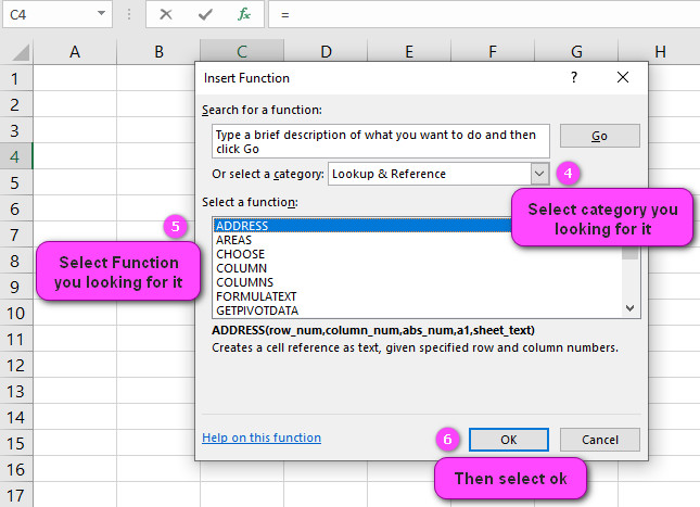
3. In the insert function tab you will see all functions.

4. Select Lookup & reference category.

5. Select GETPIVOTDATA function.

6. Then select ok

7. In function arguments Tab, you will see GETPIVOTDATA function.

8. Data field: is the name of the data field to extract data from.

9. Pivot table: is a reference to a cell or range of cells in the PivotTable that contains the data you want to retrieve.

10. Field1: field to refer to.

11. Item1: field item to refer to.

12. Field2: field to refer to.

13. You will see the result in formula result section.

Examples of GETPIVOTDATA function in excel

Here are examples of the GETPIVOTDATA function in Excel:

1.To retrieve the total sales for a specific product:

=GETPIVOTDATA("Sales",$A$1,"Product","Product A")

2.To retrieve the average sales for a specific category:

=GETPIVOTDATA("Average Sales",$A$1,"Category","Category A")

3.To retrieve the maximum sales for a specific region:

=GETPIVOTDATA("Max Sales",$A$1,"Region","North")

4.To retrieve the minimum sales for a specific month:

=GETPIVOTDATA("Min Sales",$A$1,"Month","January")

5.To retrieve the count of orders for a specific customer:

=GETPIVOTDATA("Order Count",$A$1,"Customer","Customer A")

6.To retrieve the percentage of total sales for a specific product:

=GETPIVOTDATA("% of Total Sales",$A$1,"Product","Product A")

7.To retrieve the variance of sales for a specific year:

=GETPIVOTDATA("Var Sales",$A$1,"Year",2022)

8.To retrieve the standard deviation of sales for a specific quarter:

=GETPIVOTDATA("Stdev Sales",$A$1,"Quarter","Q1")

9.To retrieve the median sales for a specific city:

=GETPIVOTDATA("Median Sales",$A$1,"City","New York")

10.To retrieve the sum of sales for a specific product and year:

=GETPIVOTDATA("Sales",$A$1,"Product","Product A","Year",2022)

Purpose of GETPIVOTDATA function in excel

The purpose of the GETPIVOTDATA function in Excel is to extract data from a pivot table based on specific criteria.

It allows users to create formulas that reference values in a pivot table without having to manually enter cell references.

The GETPIVOTDATA function retrieves data from a pivot table by specifying one or more pairs of field and item arguments, which define the criteria for the data to be retrieved.

This can be a powerful tool for creating dynamic reports that automatically update when the underlying data changes.

By using the function to extract data from a pivot table, users can create complex formulas that analyze and summarize the data in meaningful ways.

Turn off GETPIVOTDATA function in excel

The GETPIVOTDATA function can be turned off in Microsoft Excel. The GETPIVOTDATA function is a built-in feature in Excel that helps users extract data from pivot tables.

However, some users may find the function bothersome or unwanted, especially if they prefer to use cell references instead of the GETPIVOTDATA function.

To turn off the GETPIVOTDATA function in Excel:

1. Open Excel and click on the “File” tab.
2. Click on “Options” to open the “Excel Options” menu.
3. In the “Excel Options” menu, click on “Formulas”.
4. Scroll down to the “Working with Formulas” section.
5. Uncheck the box next to “Use GetPivotData functions for PivotTable references”.
6. Click “OK” to save the changes.

Once you turn off the GETPIVOTDATA function, Excel will no longer automatically insert the function when you reference cells in your pivot table.

Instead, you will need to use cell references to access the data in your pivot table.

Keep in mind that if you turn off the GETPIVOTDATA function, any existing formulas that rely on it might return errors.

Errors in GETPIVOTDATA function in excel

If your GETPIVOTDATA formula returns an error, there could be various reasons for this. Here are some of the most common issues that can cause errors with the GETPIVOTDATA function:

1. Incorrectly spelled field or item names: Ensure that you have spelled the field and item names correctly in your GETPIVOTDATA formula.
   • The field and item names are case-sensitive.
2. Referencing a cell outside of the pivot table range: Make sure that you are referencing cells within the pivot table range.
   • If you reference a cell outside the range of the pivot table, Excel will return an error.
3. Incorrect syntax in the formula: Make sure that your GETPIVOTDATA formula has the correct syntax.
   • Remember that the formula should begin with an equal sign (=), followed by the name of the function, the data field you want to retrieve, and one or more pairs of field and item arguments enclosed in quotation marks.
4. Missing arguments: Make sure that you have included all the required arguments in your GETPIVOTDATA formula. If you miss any arguments, Excel will return an error.
5. Invalid argument types: Ensure that you are using the correct argument types in your formula.
   • For example, if you are trying to retrieve data based on a date field, make sure that you enter the date in the correct format.
6. Formula not updated after changing pivot table structure: If you change the structure of your pivot table (e.g., adding or removing fields), you may need to update your GETPIVOTDATA formula accordingly.
   • You can do this by selecting the relevant fields and items again using the formula builder, rather than typing them manually.

By identifying and addressing these common issues, you can troubleshoot errors in your GETPIVOTDATA formulas and ensure that they return accurate results.

Multiple criteria in GETPIVOTDATA function in excel

you can use the GETPIVOTDATA function with multiple criteria to retrieve data from a pivot table.

The GETPIVOTDATA function is used to extract data from specific cells in a pivot table by specifying the row and column labels, as well as any additional filtering criteria.

To use the GETPIVOTDATA function with multiple criteria, you need to include all of the criteria within the same formula.

The syntax for including multiple criteria is as follows:

=GETPIVOTDATA(data_field, pivot_table, [field1, item1], [field2, item2], ...)

In this syntax, data_field is the name or index of the pivot table value that you want to retrieve, pivot_table is a reference to the pivot table cell that contains the data, and [field1, item1], [field2, item2], and so on, are pairs of field names and items that represent the filter criteria.

For example, let’s say you have a pivot table that shows sales data by region and product category, and you want to retrieve the total sales for the “West” region and the “Electronics” category. The formula would look like this:

=GETPIVOTDATA("Sales", A1, "Region", "West", "Category", "Electronics")

In this formula, “Sales” is the name of the data field, A1 is the cell reference to the pivot table, “Region” and “Category” are the field names, and “West” and “Electronics” are the filter criteria. The result will be the total sales for the specified region and category.

In summary, the GETPIVOTDATA function can be used with multiple criteria by including all of the criteria within the same formula, separated by commas.

Make more flexible GETPIVOTDATA function in excel

There are a few ways to make the GETPIVOTDATA function more flexible.

1. Use cell references for criteria:
   • Instead of hardcoding the criteria values in the formula, you can reference cell values that contain the criteria.
   • This makes it easier to change the criteria without having to modify the formula each time. For example, you could use the formula =GETPIVOTDATA("Sales", A1, "Region", B1, "Category", B2) where B1 and B2 contain the region and category criteria respectively.
2. Use wildcard characters:
   • You can use wildcard characters like asterisks (*) and question marks (?) in the criteria to match partial strings.
   • For example, if you want to retrieve data for all products that contain the word “phone” in their name, you could use the criteria "Product Name", "*phone*".
3. Use logical operators:
   • You can use logical operators like AND and OR to combine multiple criteria.
   • For example, if you want to retrieve data for products that belong to either the “Electronics” or “Office Supplies” category, you could use the formula =GETPIVOTDATA("Sales", A1, "Category", {"Electronics","Office Supplies"}).
4. Dynamically change the data field:
   • You can use a cell reference to dynamically change the data field that the GETPIVOTDATA function retrieves.
   • For example, you could use the formula =GETPIVOTDATA(B1, A1, "Region", "West", "Category", "Electronics"), where B1 contains the name of the data field to retrieve.

Overall, by using these techniques, you can make the GETPIVOTDATA function more flexible and adaptable to different scenarios.

Update my GETPIVOTDATA formula when the pivot table changes

When the layout or structure of a pivot table changes, it can affect the cell references used in the GETPIVOTDATA formula. To update the formula so that it reflects the changes made to the pivot table, you can follow these steps:

1. Identify the changes made to the pivot table:
   • Before updating the formula, it’s important to understand what changes have been made to the pivot table.
   • For example, if new fields or items have been added, or if existing fields have been moved or renamed.
2. Update the cell reference to the pivot table:
   • If the location of the pivot table has changed, you will need to update the cell reference in the GETPIVOTDATA formula to reflect the new location.
3. Verify the field names and item names:
   • If the names of fields or items in the pivot table have changed, you should update the corresponding field names and item names in the GETPIVOTDATA formula.
4. Adjust the criteria for new or modified fields:
   • If new fields have been added to the pivot table, or if existing fields have been modified, you may need to adjust the criteria in the GETPIVOTDATA formula to match the new field names and items.
5. Check for errors:
   • After updating the GETPIVOTDATA formula, you should check for any error messages that may indicate problems with the formula.
   • Common errors include #REF! or #VALUE!, which typically occur when a cell reference is incorrect or when the formula contains invalid arguments.

Overall, by following these steps, you can update your GETPIVOTDATA formula to reflect the changes made to the pivot table, ensuring that it continues to retrieve accurate data.

Use the GETPIVOTDATA function with external data sources

you can use the GETPIVOTDATA function with external data sources in Microsoft Excel.

The GETPIVOTDATA function is a powerful tool in Excel that allows you to extract specific data from a pivot table.

By default, the function references cells within the same workbook where the pivot table is located.

However, you can also use the GETPIVOTDATA function to retrieve data from an external data source such as an Access database, SQL Server, or ODBC data source. To do this, you need to create a connection between Excel and the data source.

Here are the steps to use the GETPIVOTDATA function with an external data source:

1. Click on the Data tab in the Excel ribbon.
2. In the Get External Data section, click on From Other Sources and select the type of data source you want to use.
3. Follow the prompts to connect to the data source and import the data into Excel.
4. Once you have imported the data, create a pivot table based on the external data source.
5. Use the GETPIVOTDATA function to extract data from the external data source by referencing the pivot table cells that contain the data.

Note that when using the GETPIVOTDATA function with an external data source, the reference to the pivot table cells will include the name of the external data source and its location.

This will allow Excel to correctly identify the source of the data and extract the desired information.

Related posts:

Excel DGET Function Excel ROWS Function Excel DCOUNT Function DMIN function in Excel