What is GESTEP function in Excel?
The GESTEP function is one of the Engineering functions of Excel.
It Tests whether a number is greater than a threshold value.
We can find this function in Engineering category of the insert function Tab.
How to use GESTEP function in excel
- Click on an empty cell (like F5).

2. Click on the fx icon (or press shift+F3).

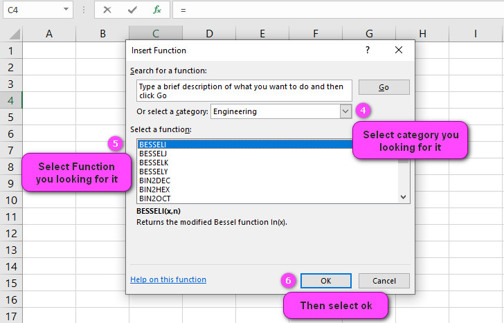
3. In the insert function tab you will see all functions.

4. Select ENGINEERING category.
5. Select GESTEP function
6. Then select ok.
7. In the function arguments Tab you will see GESTEP function.
8. Number section is the value to test against step.
9. Step section is the threshold value.
10. You will see the results in the formula result section.

Examples of GESTEP function in Excel
=GESTEP(5,2)returns 1 because 5 is greater than 2.=GESTEP(-3,0)returns 0 because -3 is less than 0.=GESTEP(B2,AVERAGE(B2:B10))returns 1 if the value in cell B2 is greater than the average of the range B2:B10, and 0 otherwise.=GESTEP(1000,MAX(A1:A100))returns 0 if the value in cell A1:A100 is greater than or equal to 1000, and 1 otherwise.=IF(GESTEP(D2,50), "Pass", "Fail")returns “Pass” if the value in cell D2 is greater than 50, and “Fail” otherwise.=SUMIFS(C2:C10,B2:B10,">="&D2,B2:B10,"<"&E2)returns the sum of the values in the range C2:C10 that fall between the values in cells D2 and E2.=COUNTIFS(B2:B100,">0",C2:C100,"<>N/A",D2:D100,"<=30",E2:E100,"<>")counts the number of rows where the value in column B is greater than 0, column C is not empty, column D is less than or equal to 30, and column E is not blank.=AVERAGEIF(B2:B10,">="&E2,C2:C10)calculates the average of the values in the range C2:C10 that correspond to values in the range B2:B10 that are greater than or equal to the value in cell E2.=SUMPRODUCT(GESTEP(B2:B10,5)*C2:C10)calculates the sum of the values in the range C2:C10 that correspond to values in the range B2:B10 that are greater than 5.=IFERROR(GESTEP(1/0,1), "Error")returns “Error” because the expression 1/0 results in a #DIV/0! error, which is handled by the IFERROR function.

Excel’s GESTEP function: What Does It Do?
The GESTEP function in Excel is a logical function that returns 1 if a number is greater than or equal to a threshold value, and 0 otherwise. It is often used in combination with other functions for data analysis and decision-making.
For example, suppose we have a list of test scores in cells A1:A10, and we want to determine which scores are above the passing grade of 70. We can use the following formula:
=GESTEP(A1:A10,70)
This will return an array of values where 1 corresponds to scores that are greater than or equal to 70, and 0 corresponds to scores that are less than 70.
Understanding Arguments in Excel’s GESTEP Function
The GESTEP function in Excel takes two arguments: the number to be compared, and the threshold value. If the number is greater than or equal to the threshold, the function returns 1; otherwise, it returns 0.
For example, suppose we want to compare the value in cell B2 to the threshold value of 5. We can use the following formula:
=GESTEP(B2,5)
This will return 1 if the value in B2 is greater than or equal to 5, and 0 otherwise.
Syntax of Excel’s GESTEP Function: Explained
The syntax of the GESTEP function in Excel is as follows:
=GESTEP(number, step)
where “number” is the value to be compared, and “step” is the threshold value.
For example, if we want to check whether the value in cell C2 is greater than or equal to 10, we can use the following formula:
=GESTEP(C2,10)
This will return 1 if the value in C2 is greater than or equal to 10, and 0 otherwise.
Learn About Return Value of Excel’s GESTEP Function
The return value of the GESTEP function in Excel is always either 1 or 0. If the number being compared is greater than or equal to the threshold value, the function returns 1; otherwise, it returns 0.
For example, suppose we want to compare the values in cells D2:D10 to a threshold value of 20. We can use the following formula:
=GESTEP(D2:D10,20)
This will return an array of values where 1 corresponds to values that are greater than or equal to 20, and 0 corresponds to values that are less than 20.
Comparing Two Lists of Values using Excel’s GESTEP Function
To compare two lists of values using the GESTEP function in Excel, we can use the SUMPRODUCT function to sum the corresponding values in the two arrays.
For example, suppose we have two lists of test scores in cells A1:A5 and B1:B5, and we want to count the number of times a score in list A is greater than or equal to the corresponding score in list B. We can use the following formula:
=SUMPRODUCT(GESTEP(A1:A5,B1:B5))
This will return the number of times a score in list A is greater than or equal to the corresponding score in list B.
Difference between GESTEP Function and GREATER THAN (>) Operator in Excel
The GESTEP function and the greater than (>) operator both compare values in Excel, but they return different types of results. The GESTEP function returns 0 or 1 based on whether the value is greater than or equal to a threshold, while the greater than operator returns a logical TRUE/FALSE value.
For example, suppose we want to check if the value in cell A1 is greater than 10 using the greater than operator. We can use the following formula:
=A1>10
This will return TRUE if the value in A1 is greater than 10, and FALSE otherwise.
On the other hand, if we want to check if the value in cell A1 is greater than or equal to 10 using the GESTEP function, we can use the following formula:
=GESTEP(A1,10)
This will return 1 if the value in A1 is greater than or equal to 10, and 0 otherwise.
Can GESTEP Function be Used with Text Values in Excel?
No, the GESTEP function in Excel cannot be used with text values. It only works with numerical values.
For example, if we have a list of grades in cells B2:B10 and we want to count the number of times a student received an “A”, we cannot use the GESTEP function. Instead, we could use the COUNTIF function as follows:
=COUNTIF(B2:B10,"A")
This will count the number of cells in the range B2:B10 that contain the letter “A”.
Counting Cells Based on a Certain Condition Using Excel’s GESTEP Function
To count the number of cells in a range that meet a certain condition using the GESTEP function in Excel, we can use the SUM function to add up the resulting array of 1’s and 0’s.
For example, suppose we have a list of temperatures in cells A2:A10, and we want to count the number of values that are greater than or equal to 100. We can use the following formula:
=SUM(GESTEP(A2:A10,100))
This will return the number of values in the range A2:A10 that are greater than or equal to 100.
Logical Operators like AND and OR with Excel’s GESTEP Function
The GESTEP function in Excel can be combined with logical operators like AND and OR to create more complex conditions for data analysis and decision-making.
For example, suppose we have a list of test scores in cells B2:B10, and we want to count the number of students who scored above 70 on both the midterm and final exams. We can use the following formula:
=SUM((GESTEP(B2:B10,70))*(B2:B10>70))
This will return the number of students who scored above 70 on both exams.
Nesting the GESTEP function within another function in Excel
The GESTEP function in Excel can be nested within other functions to perform more complex calculations based on certain conditions.
For example, suppose we have a table of sales data with columns for Date, Product ID, Units Sold, and Revenue. If we want to calculate the total revenue for a specific product sold over a certain date range, we might use the SUMIFS function in combination with the GESTEP function to filter the data based on those conditions.
We could use the following formula:
=SUMIFS(Revenue,ProductID,"A",UnitsSold,">"&0,GESTEP(Date,"06/01/2023")=1)
This will return the sum of the Revenue column where the value in the ProductID column is “A”, the value in the UnitsSold column is greater than 0, and the Date is on or after June 1, 2023.
Accuracy of Excel’s GESTEP Function
The GESTEP function in Excel is a reliable and accurate way to compare values and return either 0 or 1 based on whether the value meets a certain threshold. However, like any function, it is important to use it correctly and ensure that the data being analyzed is in the correct format.
For example, if we have a list of test scores in cells A2:A10 and we want to count the number of students who scored above 90, we can use the following formula:
=SUM(GESTEP(A2:A10,90))
This will return the number of values in the range A2:A10 that are greater than or equal to 90.
Handling Nested IF Statements with Excel’s GESTEP Function
The GESTEP function in Excel can be nested within other functions, including nested IF statements, to perform more complex calculations based on certain conditions.
For example, suppose we have a list of sales data with columns for Date, Product ID, Units Sold, and Revenue. If we want to categorize the products as “High”, “Medium”, or “Low” based on their revenue, we might use a nested IF statement in combination with the GESTEP function.
We could use the following formula:
=IF(GESTEP(Revenue,5000), "High", IF(GESTEP(Revenue,2500), "Medium", "Low"))
This will categorize the products as “High” if their revenue is greater than or equal to 5000, “Medium” if it is between 2500 and 4999, and “Low” if it is less than 2500.
Combining Excel’s GESTEP Function with Other Logical Functions
The GESTEP function in Excel can be combined with other logical functions like AND, OR, NOT, and IF to create more complex conditions and calculations.
For example, suppose we have a list of test scores in cells A2:A10 and we want to count the number of students who scored above 80 and below 90. We can use the following formula:
=SUM(GESTEP(A2:A10,80)*NOT(GESTEP(A2:A10,90)))
This will return the number of values in the range A2:A10 that are greater than or equal to 80 and less than 90.
Dynamic Ranges and Excel’s GESTEP Function
The GESTEP function in Excel can be used with dynamic ranges by using named ranges or the OFFSET function.
For example, suppose we have a table of sales data with columns for Date, Product ID, Units Sold, and Revenue, and we want to count the number of products sold in the last 30 days. We can use the OFFSET function to create a dynamic range:
=SUM(GESTEP(OFFSET(Revenue,COUNT(Revenue)-30,0,30,1),100))
This will return the number of products sold in the last 30 days where the revenue is greater than or equal to 100.
Using Excel’s GESTEP Function for Conditional Formatting
The GESTEP function in Excel can be used to apply conditional formatting to cells based on certain conditions.
For example, suppose we have a list of test scores in cells A2:A10 and we want to highlight the cells that are above the passing grade of 70. We can use the following steps:
- Select the range A2:A10
- Click on “Conditional Formatting” in the Home tab
- Select “New Rule”
- Choose “Use a formula to determine which cells to format”
- Enter the following formula:
=GESTEP(A2,70) - Choose the desired formatting options
- Click “OK”
This will highlight the cells in the range A2:A10 that are greater than or equal to 70.
Array Formulas and Excel’s GESTEP Function
The GESTEP function in Excel can be used with array formulas to apply the calculation to multiple cells at once.
For example, suppose we have a list of test scores in cells A2:A10 and we want to count the number of students who scored above 85 using an array formula. We can use the following formula:
=SUM(IF(GESTEP(A2:A10,85),1,0))
This will return the number of values in the range A2:A10 that are greater than or equal to 85.
Note that when using array formulas, it is important to press Ctrl+Shift+Enter instead of just Enter to activate the formula.
Troubleshooting Errors with Excel’s GESTEP Function
If there are errors when using the GESTEP function in Excel, it is likely due to issues with the data being analyzed. Some common errors include using the wrong argument types, using non-numeric values with the function, or referring to cells that contain errors.
For example, if we have a list of test scores in cells B2:B10 and some of the cells contain text instead of numbers, we might encounter the #VALUE! error when using the GESTEP function. To avoid this error, we can use the following formula:
=SUM(IF(ISNUMBER(B2:B10)*GESTEP(B2:B10,70),1,0))
This will return the number of cells in the range B2:B10 that contain a number and are greater than or equal to 70.
Data Validation Rules using Excel’s GESTEP Function
The GESTEP function in Excel can be used with data validation rules to restrict input based on certain conditions.
For example, suppose we want to create a data validation rule for a cell such that the value entered must be greater than or equal to 50. We can use the following formula:
=GESTEP(A1,50)
This will allow values greater than or equal to 50 and disallow values less than 50.
Non-numeric Values and Excel’s GESTEP Function
The GESTEP function in Excel only works with numerical values and cannot be used with non-numeric values like text or dates.
For example, if we have a list of grades in cells B2:B10 and we want to count the number of times a student received an “A+”, we cannot use the GESTEP function. Instead, we could use the following formula:
=COUNTIF(B2:B10,"A+")
This will count the number of cells in the range B2:B10 that contain the value “A+”.
Statistical Analysis with Excel’s GESTEP Function
The GESTEP function in Excel can be used for statistical analysis by comparing values to a certain threshold and calculating percentages or other statistics based on those comparisons.
For example, suppose we have a list of test scores in cells A2:A10 and we want to calculate the percentage of scores that are above 80. We can use the following formula:
=SUM(GESTEP(A2:A10,80))/COUNT(A2:A10)
This will return the percentage of values in the range A2:A10 that are greater than or equal to 80.
GESTEP related functions
- GROWTH function
- Use LOG function to return the logarithm of a number to the base you specify.
