HYPERLINK Function in Excel

The HYPERLINK function is one of the (Lookup & reference) functions of Excel.

it creates a shortcut or jump that opens a document stored on your hard drive, a network server, or on the internet.

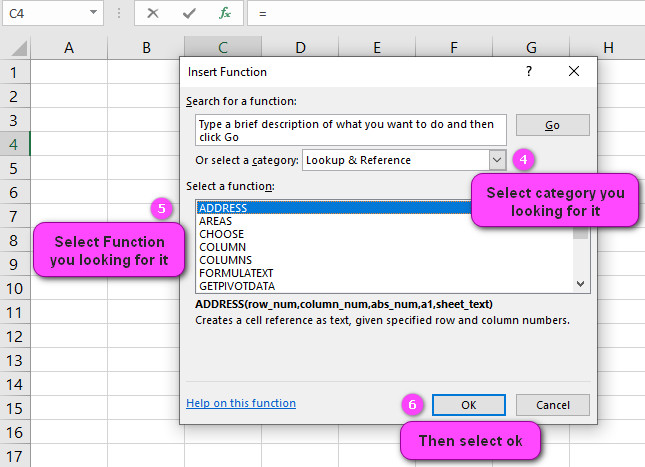
We can find this function in Lookup & reference of insert function Tab.

How to use HYPERLINK function in excel

1. Click on empty cell (like F5)

2. Click on fx on the below of font word (or press shift+F3)

3. In insert function tab you will see all functions

4. Select Lookup & reference category

5. Select HYPERLINK function

6. Then select ok

7. In function arguments Tab, you will see HYPERLINK function

8. link_location is the text giving the path and file name to the document to be opened, a hard

drive location, UNC address, or URL path.

9. Friendly_name is text or a number that is displayed in the cell. If omitted, the cell displays

the link_location text.

10. If you enter in link_location ex: “C:\Users\my\Desktop\100.xls”

11. If you enter in friendly_name ex: my excell

12. This will open (100.xls) which save in your desktop

13. You will see the result in formula result section

Examples of HYPERLINK function in excel

Sure, here are some examples of the HYPERLINK function in Excel:

1. Basic hyperlink: The simplest form of the HYPERLINK function creates a link to a web page or file. For example:

=HYPERLINK("https://www.google.com", "Google")

In this formula, the first argument is the web address for Google, and the second argument is the text that will be displayed as the hyperlink in the cell.

When the user clicks on the hyperlink, their default web browser will open and take them to Google’s homepage.

2. Email hyperlink: You can also use the HYPERLINK function to create a hyperlink that opens an email message with a pre-filled subject line and body. For example:

=HYPERLINK("mailto:sales@example.com?subject=Order Inquiry&body=Dear%20Sales%20Team,%0D%0A%0D%0AI%20am%20interested%20in%20placing%20an%20order.%20Could%20you%20please%20provide%20me%20with%20more%20information%20about%20your%20products?","Contact Sales Team")

In this formula, the first argument starts with “mailto:” to indicate that this is an email link. It includes the email address “sales@example.com“, as well as the subject line (“Order Inquiry”) and message body, which are separated by the “%0D%0A” code (which represents a new line character). The second argument is the text that will be displayed as the hyperlink in the cell.

3. Internal worksheet hyperlink: You can use the HYPERLINK function to create a hyperlink that points to a specific cell or range of cells within the same worksheet. For example:

=HYPERLINK("#Sheet1!B5:C7", "View Data")

In this formula, the first argument starts with “#” to indicate that this is a reference to a cell within the same workbook.

It includes the sheet name (“Sheet1!”) and the cell range (“B5:C7”). The second argument is the text that will be displayed as the hyperlink in the cell.

4. External worksheet or workbook hyperlink: You can also use the HYPERLINK function to create a hyperlink that points to a specific cell or range of cells in another worksheet or workbook. For example:

=HYPERLINK("[Budget.xlsx]Sheet2!A1", "View Budget")

In this formula, the first argument includes the file name (“Budget.xlsx”), the sheet name (“Sheet2!”), and the cell reference (“A1”).

The second argument is the text that will be displayed as the hyperlink in the cell. Note that the file name must be enclosed in square brackets, and the full path to the file must be included if it is not in the same folder as the current workbook.

These are just a few examples of how you can use the HYPERLINK function in Excel. The possibilities are almost endless, depending on your needs and creativity!

Create a HYPERLINK in excel

To create a hyperlink in Excel, follow these steps:

1. Select the cell or text that you want to turn into a hyperlink.

2. Right-click and select “Hyperlink” from the dropdown menu, or use the keyboard shortcut Ctrl + K.

3. In the “Insert Hyperlink” dialog box, choose the type of link you want to create.

You can link to an existing file or webpage, create a new email message, or link to a specific location within the current workbook.

4. Enter the destination URL or email address, or select the file or location you want to link to.

5. If you want to customize the display text for the hyperlink, enter it in the “Text to display” field.

6. Click “OK” to create the hyperlink.

For example, let’s say you have a list of products in column A of your Excel worksheet, and you want to create hyperlinks to their corresponding product pages on your website. You would:

1. Select the first cell in column A that contains a product name.

2. Right-click and select “Hyperlink” from the dropdown menu, or use the keyboard shortcut Ctrl + K.

3. In the “Insert Hyperlink” dialog box, select “Existing File or Web Page”.

4. Enter the URL for the product page on your website.

5. Click “OK” to create the hyperlink.

6. Repeat these steps for each product in column A.

Now, when you click on a product name in column A, Excel will open your website and take you directly to the corresponding product page.

Examples of HYPERLINK function in excel

To create a hyperlink in Excel, follow these steps:

1. Select the cell or text that you want to turn into a hyperlink.

2. Right-click and select “Hyperlink” from the dropdown menu, or use the keyboard shortcut Ctrl + K.

3. In the “Insert Hyperlink” dialog box, choose the type of link you want to create. You can link to an existing file or webpage, create a new email message, or link to a specific location within the current workbook.

4. Enter the destination URL or email address, or select the file or location you want to link to.

5. If you want to customize the display text for the hyperlink, enter it in the “Text to display” field.

6. Click “OK” to create the hyperlink.

For example, let’s say you have a list of products in column A of your Excel worksheet, and you want to create hyperlinks to their corresponding product pages on your website. You would:

1. Select the first cell in column A that contains a product name.

2. Right-click and select “Hyperlink” from the dropdown menu, or use the keyboard shortcut Ctrl + K.

3. In the “Insert Hyperlink” dialog box, select “Existing File or Web Page”.

4. Enter the URL for the product page on your website.

5. Click “OK” to create the hyperlink.

6. Repeat these steps for each product in column A.

Now, when you click on a product name in column A, Excel will open your website and take you directly to the corresponding product page.

Remove a HYPERLINK in Excel

To remove a hyperlink in Excel, follow these steps:

1. Select the cell with the hyperlink you want to remove.

2. Right-click on the cell and select “Remove Hyperlink” from the context menu.

3. The hyperlink will be removed and the cell will show only the plain text.

Alternatively, you can also remove a hyperlink by selecting the cell and pressing “Ctrl” + “K” on your keyboard to bring up the “Edit Hyperlink” dialog box.

Then click “Remove Link” and the hyperlink will be removed.

Make an image into a HYPERLINK in Excel

To make an image into a hyperlink in Excel, you can follow these steps:

1. Insert the image into your Excel worksheet by clicking on the “Insert” tab and selecting “Pictures.”
2. Select the image you want to turn into a hyperlink.
3. Right-click on the image and select “Hyperlink” from the drop-down menu.
4. In the “Insert Hyperlink” dialog box, choose “Place in This Document” from the list on the left.
5. Choose the cell you want to link to by scrolling through the list or entering the cell reference in the “Type the Cell Reference” field.
6. Click OK to close the dialog box and apply the hyperlink to the image.

Here’s an example of how to do this:

Let’s say you have an Excel spreadsheet with some data in cells A1 to B10, and you want to insert an image that links to cell A1.

To do this, you would follow these steps:

1. Click on the “Insert” tab and select “Pictures.”
2. Browse for the image you want to use and click “Insert.”
3. Once the image is inserted, click on it to select it.
4. Right-click on the image and select “Hyperlink” from the drop-down menu.
5. In the “Insert Hyperlink” dialog box, choose “Place in This Document” from the list on the left.
6. Scroll through the list to find cell A1 or type “A1” in the “Type the Cell Reference” field.
7. Click OK to close the dialog box and apply the hyperlink to the image.

Now, when someone clicks on the image, they will be taken directly to cell A1 in your Excel worksheet.

Create a clickable email address or website or file in Excel

To create a clickable email address or website or file in Excel, you can use the “Insert Hyperlink” feature. Here’s how to do it:

1. Select the cell where you want to insert the hyperlink.
2. Right-click on the cell and select “Hyperlink” from the drop-down menu, or go to the “Insert” tab and click on “Hyperlink.”
3. In the “Insert Hyperlink” dialog box, choose the type of hyperlink you want to insert:

• To create a clickable email address, choose “E-mail Address” from the list on the left. Enter the email address in the “E-mail address” field and click “OK.” You can also use the “Subject” field to add a subject line for the email.
• To create a clickable website link, choose “Existing File or Web Page” from the list on the left. Enter the URL in the “Address” field and click “OK.”
• To create a clickable link to a file, choose “Existing File or Web Page” from the list on the left. Browse to the file you want to link to and select it. Click “OK” to insert the link.

4. Once you’ve inserted the hyperlink, you can customize its display text by selecting the cell and editing its contents. For example, you could replace the email address with the words “Click here to email us” or the website URL with the name of the site.

Here are some examples:

1. To create a clickable email address in cell A1, right-click on the cell and select “Hyperlink.” In the “Insert Hyperlink” dialog box, choose “E-mail Address” and enter the email address in the “E-mail address” field. You could also add a subject line in the “Subject” field if desired. Click “OK” to insert the hyperlink. The cell will now display the email address and clicking on it will automatically open the user’s email client with a new message addressed to that email.
2. To create a clickable website link in cell A1, right-click on the cell and select “Hyperlink.” In the “Insert Hyperlink” dialog box, choose “Existing File or Web Page” and enter the URL in the “Address” field. Click “OK” to insert the hyperlink. The cell will now display the URL and clicking on it will open the website in the user’s default web browser.
3. To create a clickable link to a file in cell A1, right-click on the cell and select “Hyperlink.” In the “Insert Hyperlink” dialog box, choose “Existing File or Web Page” and browse to the file you want to link to. Select the file and click “OK” to insert the hyperlink. The cell will now display the name of the file and clicking on it will open the file in its associated application (e.g. Excel for an .xlsx file).

Create a HYPERLINK to another worksheet or workbook in Excel

To create a hyperlink to another worksheet or workbook in Excel, you can use the “Insert Hyperlink” feature. Here’s how to do it:

1. Select the cell where you want to insert the hyperlink.
2. Right-click on the cell and select “Hyperlink” from the drop-down menu, or go to the “Insert” tab and click on “Hyperlink.”
3. In the “Insert Hyperlink” dialog box, choose “Place in This Document” from the list on the left.
4. To link to a worksheet in the same workbook, choose “Worksheet” from the list on the right, then select the worksheet you want to link to from the list.
5. To link to a different workbook, choose “Workbook” from the list on the right, then browse for the workbook you want to link to and select it.
6. Once you’ve selected the worksheet or workbook, you can customize the text that appears as the hyperlink by editing the contents of the cell.

Here are some examples:

1. To create a hyperlink to another worksheet in the same workbook, select the cell where you want to insert the hyperlink, right-click on the cell, and choose “Hyperlink” from the drop-down menu. In the “Insert Hyperlink” dialog box, choose “Place in This Document” and then “Worksheet.” Select the worksheet you want to link to from the list and click “OK.” The cell will now display the name of the worksheet as a hyperlink, and clicking on it will take the user directly to that worksheet.
2. To create a hyperlink to a different workbook, select the cell where you want to insert the hyperlink, right-click on the cell, and choose “Hyperlink” from the drop-down menu. In the “Insert Hyperlink” dialog box, choose “Place in This Document” and then “Workbook.” Click the “Browse” button and browse for the workbook you want to link to. Select the workbook and click “OK” to insert the hyperlink. The cell will now display the name of the workbook as a hyperlink, and clicking on it will open that workbook.

Note: If you’re linking to a worksheet or workbook that is located in a different folder or drive than the current file, make sure to include the full file path in the hyperlink address (e.g. C:\My Documents\Workbook2.xlsx!Sheet1).

Make a HYPERLINK that goes to a specific cell in Excel

To make a hyperlink that goes to a specific cell in Excel, you can use the “Insert Hyperlink” feature. Here’s how to do it:

1. Select the cell where you want to insert the hyperlink.
2. Right-click on the cell and select “Hyperlink” from the drop-down menu, or go to the “Insert” tab and click on “Hyperlink.”
3. In the “Insert Hyperlink” dialog box, choose “Place in This Document” from the list on the left.
4. Enter the reference of the cell that you want to link to in the “Type the Cell Reference” field. You can also use the “Defined Names” and “Sheet” lists to select the cell.
5. Click OK to close the dialog box and apply the hyperlink to the cell.

Here are some examples:

1. To create a hyperlink that goes to cell A1, select the cell where you want to insert the hyperlink, right-click on the cell, and choose “Hyperlink” from the drop-down menu. In the “Insert Hyperlink” dialog box, choose “Place in This Document” and enter “A1” in the “Type the Cell Reference” field. Click “OK” to insert the hyperlink. The cell will now be underlined and displayed in blue, indicating that it is a hyperlink. Clicking on it will take the user directly to cell A1.
2. To create a hyperlink that goes to a cell in another worksheet or workbook, follow the same steps as above but include the name of the worksheet or workbook in the cell reference. For example, if you want to link to cell B2 in Sheet2 of the current workbook, you would enter “Sheet2!B2” in the “Type the Cell Reference” field. If you want to link to cell C5 in Sheet1 of a different workbook called “Book2.xlsx,” you would enter “C5” in the “Type the Cell Reference” field and then add the full file path to the workbook (e.g. “C:\Documents\Book2.xlsx!Sheet1!C5”).

Difference between a relative link and an absolute link in Excel

In Excel, there are two types of links: relative links and absolute links. The main difference between them is how the link address is interpreted and updated when the location of the linked file or worksheet changes.

A relative link is a link that refers to a cell or range in a worksheet using a path that is relative to the location of the current workbook.

In other words, the link address is based on the position of the linked file or worksheet relative to the current file.

For example, if you have a workbook called “Book1.xlsx” and it contains a relative link to a worksheet in another workbook called “Book2.xlsx,” the link address will be something like “../Book2.xlsx!Sheet1”.

If you move Book1.xlsx to a different folder or rename it, the link address will be updated automatically to reflect the new location.

An absolute link, on the other hand, is a link that uses an explicit path to refer to a file or worksheet. The link address remains the same no matter where the linked file or worksheet is located.

For example, if you have an absolute link to a worksheet in another workbook called “C:\Users\John\Documents\Book2.xlsx!Sheet1”, the link address will always be the same no matter what happens to the linked file or worksheet.

Here are some examples:

1. Relative link: Suppose you have a formula in cell A1 of “Book1.xlsx” that refers to cell B2 in “Sheet1” of “Book2.xlsx”. The formula could be written as “=SUM([Book2.xlsx]Sheet1!B2)”. If you move “Book1.xlsx” to a different folder or rename it, the link address will be updated automatically to reflect the new location of “Book2.xlsx”.
2. Absolute link: Suppose you have a formula in cell A1 of “Book1.xlsx” that refers to cell B2 in “Sheet1” of “Book2.xlsx”, using an absolute link. The formula could be written as “=SUM(‘C:\Users\John\Documents[Book2.xlsx]Sheet1’!B2)”. The link address will always point to the same location, regardless of where “Book1.xlsx” is saved.

In summary, relative links are useful when you want to create links that can be easily updated if the locations of the linked files change, while absolute links are used for links that should always point to the same location, regardless of where the current file is saved or moved.

Edit an existing HYPERLINK in Excel

To edit an existing hyperlink in Excel, you can follow these steps:

1. Select the cell that contains the hyperlink.
2. Right-click on the cell and select “Edit Hyperlink” from the drop-down menu.
3. In the “Edit Hyperlink” dialog box, you can make changes to the link address or the display text of the hyperlink. You can also choose a different type of hyperlink (e.g., email address, website, file) using the options on the left-hand side of the dialog box.
4. Once you’ve made your changes, click the “OK” button to save the updated hyperlink.

Here are some examples:

1. Suppose you have a cell in your worksheet that contains a hyperlink to a website. To edit the hyperlink, you would first select the cell and then right-click on it. From the drop-down menu, select “Edit Hyperlink.” In the “Edit Hyperlink” dialog box, you can change the URL of the website or the text that appears as the hyperlink. For example, you could change the display text to “Click here to visit our website” instead of displaying the full URL. Once you’ve made your changes, click “OK” to save the updated hyperlink.
2. Suppose you have a cell in your worksheet that contains a hyperlink to a file. To edit the hyperlink, you would select the cell and then right-click on it. From the drop-down menu, select “Edit Hyperlink.” In the “Edit Hyperlink” dialog box, you can change the path to the file or the text that appears as the hyperlink. For example, you could change the display text to the name of the file or to a more descriptive label. Once you’ve made your changes, click “OK” to save the updated hyperlink.

Note that you can also use the same steps to remove a hyperlink from a cell, by selecting the cell and then right-clicking on it and selecting “Remove Hyperlink” from the drop-down menu.

Link to a specific cell in another sheet using a HYPERLINK in Excel

To link to a specific cell in another sheet using a hyperlink in Excel, you can use the “Insert Hyperlink” feature. Here’s how to do it:

1. Select the cell where you want to insert the hyperlink.
2. Right-click on the cell and select “Hyperlink” from the drop-down menu, or go to the “Insert” tab and click on “Hyperlink.”
3. In the “Insert Hyperlink” dialog box, choose “Place in This Document” from the list on the left.
4. Click the “Bookmark” button, which is located near the bottom of the dialog box.
5. In the “Bookmark” dialog box, give the target cell a name (e.g., “TargetCell”), then click “Add.” Note that the name should be unique within the workbook.
6. Click “OK” to close the “Bookmark” dialog box, then enter the name of the target worksheet followed by an exclamation point and the cell reference (e.g., “Sheet2!TargetCell”) in the “Type the Cell Reference” field.
7. Click “OK” to close the “Insert Hyperlink” dialog box and apply the hyperlink to the cell.

Here are some examples:

1. To create a hyperlink that goes to cell A1 on Sheet2, select the cell where you want to insert the hyperlink, right-click on the cell, and choose “Hyperlink” from the drop-down menu. In the “Insert Hyperlink” dialog box, choose “Place in This Document,” then click the “Bookmark” button. In the “Bookmark” dialog box, enter “TargetCell” as the name for cell A1, then click “Add.” Next, enter “Sheet2!TargetCell” in the “Type the Cell Reference” field, then click “OK” to close both dialog boxes. The cell will now display the name of the target sheet followed by the cell reference, and clicking on it will take the user directly to cell A1 on Sheet2.
2. To create a hyperlink that goes to cell B4 on Sheet3, select the cell where you want to insert the hyperlink, right-click on the cell, and choose “Hyperlink” from the drop-down menu. In the “Insert Hyperlink” dialog box, choose “Place in This Document,” then click the “Bookmark” button. In the “Bookmark” dialog box, enter “TargetCell” as the name for cell B4, then click “Add.” Next, enter “Sheet3!TargetCell” in the “Type the Cell Reference” field, then click “OK” to close both dialog boxes. The cell will now display the name of the target sheet followed by the cell reference, and clicking on it will take the user directly to cell B4 on Sheet3.

Format the appearance of HYPERLINKS in Excel

To format the appearance of hyperlinks in Excel, you can use the “Cell Styles” feature. Here’s how to do it:

1. Select the cell or range of cells that contains the hyperlink(s).
2. Go to the “Home” tab and click on the “Cell Styles” button in the “Styles” group.
3. In the “Cell Styles” gallery, click on the style that you want to apply to the hyperlink(s). Note that some styles may have a special formatting for hyperlinks, such as underlining and color.
4. If you want to create a custom style for hyperlinks, right-click on one of the existing styles in the “Cell Styles” gallery and select “Modify.” In the “Modify Style” dialog box, you can change the formatting options, including font, fill, border, and number format, for both the normal and hover states of the hyperlink.
5. Once you’ve made your changes, click “OK” to save the new style.

Here are some examples:

1. To apply a predefined style to a cell or range of cells that contain hyperlinks, select the cell or range, go to the “Home” tab, and click on the “Cell Styles” button. Choose a style from the gallery, such as “Hyperlink” or “Linked Cell,” which includes special formatting for hyperlinks, such as blue font and underlining. The selected style will be applied to all cells containing hyperlinks in the selected range.
2. To create a custom style for hyperlinks, right-click on an existing style in the “Cell Styles” gallery and select “Modify.” In the “Modify Style” dialog box, you can customize the font, fill, border, and number format for both the normal and hover states of the hyperlink. For example, you could change the font color to red and remove the underline from the normal state, while adding a blue background and bold font to the hover state. Once you’re satisfied with the formatting options, click “OK” to save the new style.

Note that you can also change the default hyperlink formatting options by going to the “File” tab, selecting “Options,” then “Proofing,” and clicking on the “AutoCorrect Options” button.

In the “AutoCorrect” dialog box, go to the “AutoFormat As You Type” tab and check or uncheck the options under “Replace as you type” to enable or disable hyperlink formatting, such as underlining and changing the font color.

Formula to create dynamic HYPERLINKS in Excel

To create dynamic hyperlinks in Excel, you can use a combination of the “HYPERLINK” function and other Excel functions to build the hyperlink address dynamically based on the values in other cells. Here’s an example formula:

=HYPERLINK(CONCATENATE("https://www.example.com/?search=",A1),"Click here to search for "&A1)

In this formula, we are using the CONCATENATE function to combine the search term in cell A1 with the base URL “https://www.example.com/?search=“.

The result is a complete URL that includes the search term.

We then use the HYPERLINK function to create the actual hyperlink, using the dynamically generated URL as the link address. We also include some text (in quotes) that will be displayed as the link text.

When you enter this formula into a cell, it will display as a hyperlink, where the link text is “Click here to search for

” (where is the value in cell A1), and clicking on the link will take the user to the dynamically generated URL.

Here are some additional examples of formulas that use dynamic hyperlinks:

• To create a hyperlink to a specific cell in another worksheet, you can use a formula like this:

=HYPERLINK("#"&"'Sheet2'!B4","Go to B4 in Sheet2")

This formula creates a hyperlink that goes to cell B4 in a worksheet called “Sheet2”. The “#&” portion of the formula tells Excel that this is a reference to a cell within the same workbook, and the “&” symbol concatenates the sheet name (“‘Sheet2’!”) with the cell reference (“B4”).

• To create a hyperlink that opens an email message with a pre-filled subject line and body, you can use a formula like this:

=HYPERLINK("mailto:info@example.com?subject="&A1&"&body="&B1,"Click here to send email")

This formula creates a hyperlink that opens the user’s default email client and pre-fills the subject line with the value in cell A1 and the body of the message with the value in cell B1.

The “mailto:” prefix tells Excel that this is an email link, and the “&” symbol concatenates the email address (“info@example.com“), the subject line (“&subject=”&A1), and the message body (“&body=”&B1).

Follow a HYPERLINK in Excel

To follow a hyperlink in Excel, you can simply click on the cell that contains the hyperlink. Here’s how it works:

1. When you move the mouse pointer over a cell that contains a hyperlink, the pointer will change to indicate that the cell contains a hyperlink.
2. Click on the cell to follow the hyperlink. If the hyperlink is a web address or URL, your default web browser will open and take you to the website. If the hyperlink points to a file, such as a Word document or PDF, the corresponding application will open the file. If the hyperlink points to a specific cell or range of cells in another worksheet or workbook, Excel will take you to that location.
3. To return to the original worksheet or workbook, use the “Back” button in your web browser or use the navigation commands in Excel to go back to the previous sheet.

Here are some examples:

1. Suppose you have a worksheet that contains hyperlinks to different websites. To follow a hyperlink, simply click on the cell that contains the hyperlink. For example, if you have a hyperlink in cell A1 that points to “https://www.example.com/“, clicking on the cell will launch your default web browser and take you to the website.
2. Suppose you have a worksheet that contains hyperlinks to files on your computer. To follow a hyperlink, click on the cell that contains the hyperlink. For example, if you have a hyperlink in cell A2 that points to a Word document called “Document1.docx”, clicking on the cell will open the file in Microsoft Word (assuming that Word is installed on your computer).
3. Suppose you have a worksheet that contains hyperlinks to other worksheets or workbooks. To follow a hyperlink, click on the cell that contains the hyperlink. For example, if you have a hyperlink in cell B3 that points to cell A1 in a worksheet called “Sheet2”, clicking on the cell will take you to that location in “Sheet2”.

HYPERLINKS to create a table of contents in Excel

To create a Table of Contents (TOC) in Excel using hyperlinks, you can follow these steps:

1. Create the headings for each section of your worksheet that you want to include in the TOC. For example, if you have a worksheet that contains data on different products, you could create headings for each product category, such as “Electronics”, “Clothing”, and “Toys”.
2. Next, create a separate sheet where you will insert the hyperlink for each heading. This sheet will serve as your Table of Contents. You can name this sheet “TOC” or something descriptive.
3. In the first cell of your “TOC” sheet, type the text that you want to use for the hyperlink, such as “Electronics”. Select the text and right-click on it to bring up the context menu. Choose “Hyperlink” from the options.
4. In the “Insert Hyperlink” dialog box, choose “Place in This Document” from the list on the left-hand side. Then, select the destination sheet that contains the corresponding section heading, such as “Sheet1” for the “Electronics” category. Finally, enter the cell reference for the heading, such as “A1” for the “Electronics” heading.
5. Click “OK” to create the hyperlink. Repeat this process for each section heading that you want to include in your Table of Contents.
6. When you’re finished creating all the hyperlinks for the TOC, you can add any additional formatting, such as applying colors or borders to the cells, and adjust the layout to suit your needs.

Here are some examples:

Suppose you have a worksheet that contains data on different products, with each product belonging to one of three categories: Electronics, Clothing, and Toys.

To create a Table of Contents for this worksheet, you can follow these steps:

1. Create headings for each category in the worksheet, such as “Electronics” in cell A1, “Clothing” in cell A5, and “Toys” in cell A9.
2. Create a new sheet called “TOC”.
3. In cell A1 of the “TOC” sheet, type “Electronics” (without quotes).
4. Select the text “Electronics” and right-click on it to bring up the context menu. Choose “Hyperlink” from the options.
5. In the “Insert Hyperlink” dialog box, choose “Place in This Document” from the list on the left-hand side. Then, select “Sheet1” for the destination sheet and enter “A1” for the cell reference.
6. Click “OK” to create the hyperlink.
7. Repeat this process for the other two category headings, linking them to cells A5 and A9 respectively.
8. Add any additional formatting and adjust the layout of the TOC sheet as desired.

Now, when you click on the link for “Electronics” in the TOC sheet, Excel will take you to the “Electronics” section of the main worksheet.

Similarly, clicking on the links for “Clothing” and “Toys” will take you to their corresponding sections. With this method, you can easily navigate between different sections of your worksheet using hyperlinks.

Prevent HYPERLINKS from being automatically created in Excel

Excel has an AutoFormat feature that automatically creates hyperlinks for certain types of data, such as web addresses and email addresses.

If you don’t want hyperlinks to be automatically created in your Excel workbook, you can turn off this feature by following these steps:

1. Click on the “File” tab in the ribbon.
2. Click on “Options” at the bottom of the left-hand panel.
3. In the “Excel Options” dialog box, click on “Proofing” in the left-hand panel.
4. Click on the “AutoCorrect Options” button on the right-hand side.
5. In the “AutoCorrect” dialog box, go to the “AutoFormat As You Type” tab.
6. Uncheck the boxes next to “Internet and network paths with hyperlinks” and “Replace as you type > Hyperlinks”.
7. Click “OK” to save your changes.

After you make these changes, Excel will no longer create hyperlinks automatically for web addresses or email addresses. However, you can still manually create hyperlinks using the “Hyperlink” function or the right-click menu.

Here are some examples:

Suppose you have a worksheet that contains a web address in cell A1, but you don’t want Excel to automatically create a hyperlink for it.

To prevent automatic hyperlink creation, you can follow these steps:

1. Click on the “File” tab in the ribbon.
2. Click on “Options” at the bottom of the left-hand panel.
3. In the “Excel Options” dialog box, click on “Proofing” in the left-hand panel.
4. Click on the “AutoCorrect Options” button on the right-hand side.
5. In the “AutoCorrect” dialog box, go to the “AutoFormat As You Type” tab.
6. Uncheck the box next to “Internet and network paths with hyperlinks”.
7. Click “OK” to save your changes.

Now, when you enter a web address in a cell, Excel will not automatically create a hyperlink for it. If you want to create a hyperlink manually, you can use the “Hyperlink” function or the right-click menu.

Note that turning off automatic hyperlink creation will affect all workbooks in Excel, not just the current one. If you only want to turn off automatic hyperlink creation for a specific workbook, you can use the second method described below.

Another method to prevent automatic hyperlink creation is to format the cells as plain text. To do this, select the cells where you don’t want hyperlinks to be created, right-click on them, and choose “Format Cells” from the context menu.

In the “Format Cells” dialog box, go to the “Number” tab and select “Text” from the list of categories.

Click “OK” to apply the formatting. Now, when you enter data into these cells, Excel will treat them as plain text and will not automatically create hyperlinks for them.