What is IMABS function in Excel?
The IMABS function is one of the Engineering functions of Excel.
It Returns the absolute value (modulus) of a complex number.
We can find this function in ENGINEERING of insert function Tab.
How to use IMABS function in excel
- Click on an empty cell (like F5).

2. Click on the fx icon (or press shift+F3).

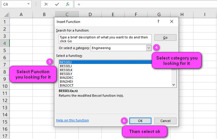
3. In the insert function tab you will see all functions.

4. Select ENGINEERING category.
5. Select IMABS function
6. Then select ok.
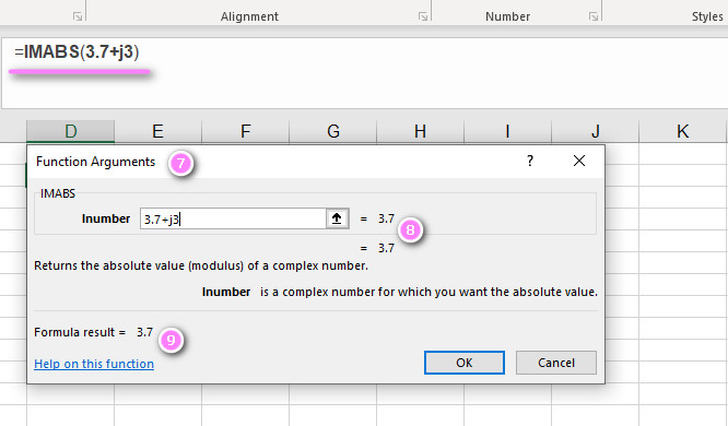
7. In the function arguments Tab you will see IMABS function.
8. Number is a complex number for which you want the absolute value.
9. You will see the results in the formula result section.
Examples of IMABS function in Excel
- =IMABS(3+4i) returns 5, as the absolute value of 3+4i is 5.
- =IMABS(-2-6i) returns 6.32455532, as the absolute value of -2-6i is approximately 6.32.
- =IMABS(0+7i) returns 7, as the absolute value of 0+7i is 7.
- =IMABS(1+i) returns 1.41421356, as the absolute value of 1+i is approximately 1.41.
- =IMABS(-5+12i) returns 13, as the absolute value of -5+12i is 13.
- =IMABS(9i) returns 9, as the absolute value of 9i is 9.
- =IMABS(2) returns 2, as the absolute value of 2 is 2.
- =IMABS(-3) returns 3, as the absolute value of -3 is 3.
- =IMABS(-2-2i) returns 2.82842712, as the absolute value of -2-2i is approximately 2.83.
- =IMABS(4+3i) returns 5, as the absolute value of 4+3i is 5.
“IMABS Function in Excel: What it Stands For and How to Use It”
The IMABS function in Excel stands for “Imaginary Absolute” and is used to return the absolute value (or modulus) of a complex number. The syntax for the IMABS function is as follows:
=IMABS(inumber)
Here, “inumber” denotes the complex number for which you want to find the absolute value.
For example, if you have the complex number -3+4i in cell A1, you can use the following formula in cell B1 to find its absolute value:
=IMABS(A1)
This will return the value 5, which is the absolute value of the complex number -3+4i.
“Mastering the Syntax of the IMABS Function in Excel”
To master the syntax of the IMABS function in Excel, you need to understand how complex numbers are represented in Excel. In Excel, complex numbers are represented using the format “x+yi”, where x and y are real numbers and i denotes the imaginary unit.
When using the IMABS function, you need to ensure that the argument passed to the function is a valid complex number in this format. If the argument is not a valid complex number, the function will return a #VALUE! error.
For example, if you try to use the IMABS function on a cell containing the text “hello world”, Excel will return a #VALUE! error since “hello world” is not a valid complex number.
“Understanding Complex Numbers for IMABS Function in Excel”
To use the IMABS function in Excel, you need to have a basic understanding of complex numbers. A complex number is a number that can be expressed in the form a+bi, where a and b are real numbers and i is the imaginary unit, which is defined as the square root of -1.
For example, the number 3+4i is a complex number, where 3 is the real part and 4i is the imaginary part.
The IMABS function in Excel is used to find the absolute value of a complex number, which is defined as the distance between the origin and the point representing the complex number in the complex plane.
“Entering Complex Numbers into the IMABS Function in Excel”
To use the IMABS function in Excel, you need to enter a valid complex number as the argument for the function.
For example, if you want to find the absolute value of the complex number 2+3i, you can use the following formula:
=IMABS(2+3i)
Alternatively, you can reference a cell containing a complex number as the argument for the function. For example, if cell A1 contains the complex number 2+3i, you can use the following formula:
=IMABS(A1)
This will return the absolute value of the complex number in cell A1.
“Discovering What the IMABS Function Returns in Excel”
The IMABS function in Excel returns the absolute value (or modulus) of a complex number. The absolute value of a complex number is defined as the distance between the origin and the point representing the complex number in the complex plane.
For example, if you have the complex number 3-4i, the absolute value is equal to the square root of (3^2 + (-4)^2), which is equal to 5. Therefore, if you use the following formula in Excel:
=IMABS(3-4i)
Excel will return the value 5, which is the absolute value of the complex number 3-4i.
“What Happens When Non-Complex Numbers are Used with IMABS Function in Excel?”
When non-complex numbers are used as the argument for the IMABS function in Excel, the function returns a #VALUE! error. This is because the IMABS function is specifically designed to work only with complex numbers.
For example, if you use the following formula:
=IMABS(5)
Excel will return a #VALUE! error since 5 is not a complex number.
“Using Arrays and Ranges of Cells with the IMABS Function in Excel”
The IMABS function in Excel can be used on arrays and ranges of cells, just like any other function. When used on an array or range of cells, the IMABS function returns an array of absolute values.
For example, let’s say you have a range of cells A1:A5, which contains the following complex numbers:
3+4i -2-6i 7+2i -8-1i 2+9i
To find the absolute value of each of these complex numbers using the IMABS function, you can use the following formula:
=IMABS(A1:A5)
This will return an array of absolute values corresponding to each of the complex numbers in the range A1:A5.
“ABS vs IMABS Functions in Excel: What’s the Difference?”
The ABS and IMABS functions in Excel both calculate the absolute value of a number, but they are used for different types of numbers. The ABS function is used for real numbers, while the IMABS function is used for complex numbers.
For example, if you have the number -5 in cell A1, you can use the ABS function to find its absolute value as follows:
=ABS(A1)
This will return the value 5.
On the other hand, if you have the complex number -2+3i in cell A1, you can use the IMABS function to find its absolute value as follows:
=IMABS(A1)
This will return the value approximately 3.61.
“Combining the IMABS Function with Other Functions in Excel”
The IMABS function in Excel can be combined with other functions to perform more complex calculations. For example, you can use the IMABS function with the SUM function to find the sum of the absolute values of a range of complex numbers.
For example, let’s say you have a range of cells A1:A5, which contains the following complex numbers:
3+4i -2-6i 7+2i -8-1i 2+9i
To find the sum of the absolute values of these complex numbers, you can use the following formula:
=SUM(IMABS(A1:A5))
This will return the value approximately 41.59.
“Finding Absolute Value of a Real Number in Excel: Is There an Equivalent Function?”
The ABS function in Excel is used to find the absolute value of a real number, which is equivalent to the magnitude of the number. The syntax for the ABS function is as follows:
=ABS(number)
Here, “number” denotes the real number for which you want to find the absolute value.
For example, if you have the number -7 in cell A1, you can use the following formula in cell B1 to find its absolute value:
=ABS(A1)
This will return the value 7, which is the absolute value of the number -7.
“Working with Negative Complex Numbers in the IMABS Function in Excel”
The IMABS function in Excel can be used on negative complex numbers, just like positive complex numbers. When a negative complex number is used as the argument for the IMABS function, the function returns the absolute value of the complex number.
For example, let’s say you have the complex number -3-4i in cell A1. You can use the following formula in cell B1 to find its absolute value:
=IMABS(A1)
This will return the value 5, which is the absolute value of the complex number -3-4i.
“Using the IMABS Function to Find the Magnitude of Vectors in Excel”
The IMABS function in Excel can be used to find the magnitude of vectors. A vector is a quantity that has both magnitude and direction. In two-dimensional space, a vector can be represented as a complex number.
For example, if you have a vector represented by the complex number 3+4i, you can use the IMABS function to find its magnitude as follows:
=IMABS(3+4i)
This will return the value 5, which is the magnitude of the vector represented by the complex number 3+4i.
“Accuracy of the IMABS Function in Excel: What You Need to Know”
The accuracy of the IMABS function in Excel depends on the precision of the arguments passed to the function. If the arguments are not precise enough, the calculated result may be less accurate than expected.
To ensure maximum accuracy when using the IMABS function, it’s important to use the correct syntax when entering complex numbers. Complex numbers should be entered using the format “x+yi”, where x and y are real numbers and i denotes the imaginary unit.
Additionally, it’s important to note that the IMABS function returns the absolute value of a complex number, which is calculated as the distance from the origin to its point in the complex plane. Therefore, the result may not be the same as the magnitude of a vector, which is calculated as the length of the vector.
“Incorporating the IMABS Function in VBA Code in Excel”
The IMABS function in Excel can also be used in VBA code. To use the IMABS function in VBA code, you simply need to call the function and pass the complex number as an argument.
For example, let’s say you have the complex number 2+3i stored in a variable called “myComplexNum”. You can use the IMABS function to find its absolute value in VBA code as follows:
Dim myComplexNum As Variant myComplexNum = 2 + 3 * WorksheetFunction.Imaginary(1) MsgBox WorksheetFunction.IMABS(myComplexNum)
This will display a message box with the value approximately 3.61, which is the absolute value of the complex number 2+3i.
“Excel Versions That Support the IMABS Function: A Comprehensive Guide”
The IMABS function was first introduced in Excel 2003 and is available in all subsequent versions of Excel, including Excel 2010, Excel 2013, Excel 2016, Excel 2019, and Excel for Office 365.
If you’re using an older version of Excel that does not support the IMABS function, you can still find the absolute value of a complex number by calculating the square root of the sum of the squares of the real and imaginary parts. For example, if you have the complex number 3+4i, you can find its absolute value using the following formula:
=SQRT(3^2+4^2)
This will return the value 5, which is the absolute value of the complex number 3+4i.
“Using the IMABS Function in Excel to Calculate Distance Between Points in a Complex Plane”
In the complex plane, the distance between two points can be calculated using the absolute value of the difference between the two points. The IMABS function in Excel can be used to calculate this distance.
For example, let’s say you have two points represented by the complex numbers 3+4i and -2-6i. You can use the following formula to find the distance between these two points:
=IMABS((3+4i)-(-2-6i))
This will return the value approximately 10.3, which is the distance between the two points.
“Modulus of a Complex Number: Finding it with the IMABS Function in Excel”
The modulus of a complex number is another term for its absolute value or magnitude. The IMABS function in Excel can be used to find the modulus of a complex number.
For example, let’s say you have the complex number 2+3i. You can use the following formula to find its modulus:
=IMABS(2+3i)
This will return the value approximately 3.61, which is the modulus of the complex number 2+3i.
“IMABS Function in Excel: Case-Sensitive or Not?”
The IMABS function in Excel is not case-sensitive, which means that you can use uppercase or lowercase letters when entering the function name.
For example, both =IMABS(A1) and =imabs(A1) will work the same way in Excel.
“Calculating Hypotenuse Length with the IMABS Function in Excel”
The hypotenuse of a right triangle can be calculated using the Pythagorean theorem, which states that the square of the length of the hypotenuse is equal to the sum of the squares of the lengths of the other two sides.
In the complex plane, the hypotenuse of a right triangle with legs represented by two complex numbers can be calculated using the IMABS function in Excel.
For example, let’s say you have a right triangle with legs represented by the complex numbers 3+4i and 4-3i. You can use the following formula to find the length of the hypotenuse:
=IMABS((3+4i)-(4-3i))
This will return the value approximately 7.81, which is the length of the hypotenuse.
“Rounding Results of the IMABS Function in Excel: Tips and Tricks”
The IMABS function in Excel returns a numeric value, which can be rounded using the ROUND function in Excel.
For example, if you have the complex number -2-3i and you want to find its absolute value rounded to one decimal place, you can use the following formula:
=ROUND(IMABS(-2-3i),1)
This will return the value 3.61, which is the absolute value of the complex number -2-3i rounded to one decimal place.
Additionally, you can format cells in Excel to display a certain number of decimal places, which can affect how the result of the IMABS function is displayed. To do this, select the cell or range of cells containing the result, then click the “Number” format dropdown menu in the “Home” tab of the ribbon and choose the desired decimal format.
IMABS related functions
- Use COMPLEX function to convert real and imaginary coefficients into complex numbers.
- IMREAL function
- Use IMAGINARY function to return the imaginary coefficient of a complex number.
- IMARGUMENT function
