What is IMCOS function in Excel?
The IMCOS function is one of the Engineering functions of Excel.
It Returns the cosine of a complex number.
We can find this function in Engineering category of the insert function Tab.
How to use IMCOS function in excel
- Click on an empty cell (like F5).

2. Click on the fx icon (or press shift+F3).

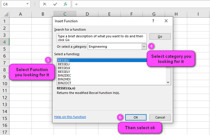
3. In the insert function tab you will see all functions.

4. Select ENGINEERING category.
5. Select IMCOS function
6. Then select ok.
7. In the function arguments Tab you will see IMCOS function.
8. Inumber section is a complex number for which you want the cosine.
9. You will see the results in the formula result section.

Examples of IMCOS function in Excel
- To find the cosine of an angle in radians, use the formula =COS(angle).
- To find the cosine of 45 degrees, which is equivalent to pi/4 radians, use the formula =COS(RADIANS(45)).
- To find the cosine of an angle in degrees, convert it to radians using the RADIANS function and then use the COS function. For example, to find the cosine of 60 degrees, use the formula =COS(RADIANS(60)).
- To find the cosine of a negative angle, simply enter the negative value into the COS function. For example, to find the cosine of -30 degrees, use the formula =COS(RADIANS(-30)).
- To calculate the cosine of an angle using a cell reference, enter the cell reference containing the angle into the COS function. For example, if the angle is in cell A1, use the formula =COS(A1).
- To calculate the cosine of multiple angles at once, enter the angles into separate cells and then use the COS function with the appropriate cell references.
- To plot the cosine wave in Excel, enter the angle values into a column, use the COS function with the corresponding values in another column, and then create a line chart.
- The domain of the COS function is all real numbers, so the function will return a value for any input. However, if the input is not in radians, you must convert it using the RADIANS function first.
- The COS function is used frequently in trigonometry and geometry problems, as well as in physics and engineering calculations.
- The COS function can also be used in combination with other functions, such as the SUM and IF functions, to perform more complex calculations involving cosine values.

Excel’s COS function: Syntax and Usage Explained
The COS function in Excel calculates the cosine of an angle given in radians. The syntax for the COS function is =COS(number), where number is the angle in radians.
For example, to find the cosine of 60 degrees in Excel, first convert it to radians using the RADIANS function: =COS(RADIANS(60)). This formula returns the value of 0.5.
Range of Values Returned by Excel’s COS Function: What You Need to Know
The range of values that the COS function can return in Excel is -1 to 1. If the input angle is outside this range, the function will return a #NUM! error.
For example, if we enter =COS(90) into a cell in Excel, the function will return the value of -0.44807361612917, since 90 degrees is equivalent to pi/2 radians.
Converting Degrees to Radians for the COS Function in Excel: Tips and Tricks
To use the COS function in Excel with angles measured in degrees, you must first convert the angle to radians using the RADIANS function.
For example, to find the cosine of 45 degrees in Excel, use the formula =COS(RADIANS(45)), which returns the value of 0.707106781186548.
ACOS vs. COS Function in Excel: Understanding the Difference
The COS function in Excel calculates the cosine of an angle, while the ACOS function calculates the inverse cosine of a value. The ACOS function is used to find the angle whose cosine is equal to a given value.
For example, to find the angle whose cosine is 0.5 in Excel, use the formula =ACOS(0.5), which returns the value of 1.0471975511966 radians (or approximately 60 degrees).
The Domain of the COS Function in Excel: A Complete Guide for Users
The domain of the COS function in Excel is all real numbers. However, if the input angle is not in radians, you must first convert it using the RADIANS function.
For example, to find the cosine of -45 degrees in Excel, use the formula =COS(RADIANS(-45)), which returns the value of 0.707106781186548.
How Excel Calculates the Cosine of an Angle: An Overview
Excel calculates the cosine of an angle using a series expansion approximation. The more terms included in the series, the more accurate the result will be.
For example, to find the cosine of 45 degrees in Excel, use the formula =COS(RADIANS(45)). Excel calculates the result using its built-in series expansion approximation and returns the value of 0.707106781186548.
Using Excel’s COS Function with Complex Numbers: What You Should Know
The COS function in Excel cannot be used with complex numbers. If you attempt to use it with a complex number, the function will return a #NUM! error.
For example, if we enter =COS(2+3i) into a cell in Excel, the function will return a #NUM! error.
Handling Errors in Excel’s COS Function: Blank or Text Input
If the input to the COS function in Excel is blank or contains text, Excel will return a #VALUE! error.
For example, if we enter =COS("") or =COS("text") into a cell in Excel, the function will return a #VALUE! error.
COS vs. COSH Function in Excel: Key Differences Explained
The COS function in Excel calculates the cosine of an angle, while the COSH function calculates the hyperbolic cosine of a value.
For example, to find the hyperbolic cosine of 2 in Excel, use the formula =COSH(2), which returns the value of 3.76219569108363.
Non-Numeric Values and Excel’s COS Function: What You Should Avoid
The COS function in Excel can only be used with numeric values. If you attempt to use it with non-numeric values, the function will return a #VALUE! error.
For example, if we enter =COS(TRUE) or =COS(FALSE) into a cell in Excel, the function will return a #VALUE! error.
The Inverse Function of the COS Function in Excel: Meet the ACOS Function
The ACOS function is the inverse function of the COS function in Excel. It returns the angle whose cosine is equal to a specified value. The syntax of the ACOS function is =ACOS(number), where number is the cosine value.
For example, if we want to find the angle whose cosine is 0.5, we can use the formula =ACOS(0.5), which returns the value of 1.0471975511966 radians (or approximately 60 degrees).
Cosine Function Period: What It Is and How It Influences Your Calculations
The period of the cosine function is 2π. This means that for any given x, cos(x) = cos(x + 2π). The period of the function can influence your calculations when dealing with periodic phenomena.
For example, if we want to graph the cosine function from -π to π in Excel, we can use the formula =COS(A1) in cell B1, where A1 contains the value of -π. We can then copy this formula to cells B2 through B21, incrementing the angle by π/10 each time. We will see that the graph repeats itself after every 2π interval.
Excel’s COS Function in Array Formulas: Tips and Best Practices
When using the COS function in an array formula in Excel, it is important to enter it as an array formula using the Ctrl + Shift + Enter key combination. This will allow the function to be applied to multiple cells at once, rather than just one.
For example, if we want to find the cosine of multiple angles in an array formula, we can use the formula {=COS(A1:A3)}, where cells A1 through A3 contain the angles in radians. When we enter this formula using the Ctrl + Shift + Enter key combination, Excel will automatically apply the function to all three cells.
Derivative of the Cosine Function: What It Means for Your Work in Excel
The derivative of the cosine function is equal to negative sine of x. This means that when graphing the cosine function, the slope at any given point x is equal to negative sine of x.
For example, if we want to find the slope of the cosine function at x = π/2, we can use the formula =-SIN(PI()/2), which returns the value of -1.
Graphing the Cosine Function in Excel: A Quick Guide
To graph the cosine function in Excel, first create a column of x values representing the domain of the function. Then create a column of y values representing the cosine of each x value. Finally, plot the x and y values on a line graph.
For example, to graph the cosine function from -π to π in Excel, create a column of x values ranging from -π to π in increments of π/10. Then create a column of y values using the formula =COS(A1) in cell B1, where A1 contains the first x value. Copy this formula to cells B2 through B21, incrementing the angle by π/10 each time. Finally, select both columns and insert a line graph to visualize the function.
Amplitude of the Cosine Function: Understanding Its Importance in Excel
The amplitude of the cosine function is the distance between the maximum and minimum values of the function. In Excel, the amplitude of the function can be used to normalize data or to find peaks and valleys in a dataset.
For example, if we want to find the amplitude of the cosine function from -π to π in Excel, we can use the formula =ABS(MAX(COS(A1:A21))) - ABS(MIN(COS(A1:A21))), where cells A1 through A21 contain the angles in radians. This formula returns the value of 2.
Phase Shift of the Cosine Function: What It Is and When to Use It
The phase shift of the cosine function is the horizontal displacement of the function relative to its usual position. This shift can be used to adjust the starting point of a periodic waveform.
For example, if we want to graph the cosine function with a phase shift of π/4 in Excel, we can use the formula =COS(A1-PI()/4) in cell B1, where A1 contains the angle in radians. We can then copy this formula to cells B2 through B21, incrementing the angle by π/10 each time. We will see that the graph starts at x = π/4 instead of the usual x = 0.
Solving Right Triangles with Excel’s COS Function: A Beginner’s Guide
The COS function in Excel can be used to solve right triangles, where one angle and one side length are known. To find the length of an unknown side, multiply the length of the known side by the cosine of the known angle.
For example, if we have a right triangle with an angle of 30 degrees and a hypotenuse of 10 units, we can use the formula =COS(RADIANS(30))*10 to find the length of the adjacent side. This formula returns the value of 8.66025404.
SEC vs. COS Function in Excel: What They Do and How to Choose Between Them
The SEC function in Excel calculates the secant of an angle, which is equal to 1/cosine of the angle. The COS function calculates the cosine of an angle. Which function to use depends on the specific calculation being performed.
For example, if we want to find the length of the hypotenuse of a right triangle given the lengths of the adjacent and opposite sides, we can use the formula =SEC(RADIANS(45)) * A1, where A1 contains the length of the adjacent side. This formula returns the length of the hypotenuse. However, if we want to find the angle between two lines, we would use the COS function instead.
Calculation Mode and Excel’s COS Function: Is There a Connection?
Excel’s calculation mode determines how formulas are calculated in a workbook. The connection with the COS function is that the calculation mode can affect the accuracy of the function’s results in some cases.
For example, if we have a workbook with many complex formulas and the calculation mode is set to automatic, the COS function may not have enough processing power to calculate its result accurately. In this case, changing the calculation mode to manual and recalculating the workbook can help improve the accuracy of the COS function’s results.
IMCOS related functions
- Use IMCOSH function to return the hyperbolic cosine of a complex number.
- Use IMSIN function to return the sine of a complex number.
- Use IMCOT function to return the cotangent of a complex number.
- Use IMTAN function to return the tangent of a complex number.
