Excel IMPRODUCT Function

What is IMPRODUCT function in Excel?

The IMPRODUCT function is one of the Engineering functions of Excel.

It Returns the product of 1 to 255 complex numbers.

We can find this function in Engineering category of the insert function Tab.

How to use IMPRODUCT function in excel

1. Click on an empty cell (like F5).

2. Click on the fx icon (or press shift+F3).

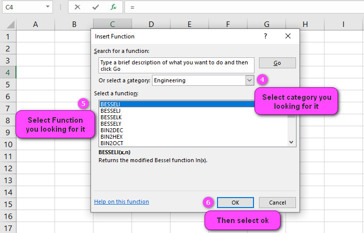
3. In the insert function tab you will see all functions.

4. Select ENGINEERING category.

5. Select IMPRODUCT function

6. Then select ok.

7. In function arguments Tab you will see IMPRODUCT function.

8. Inumber1: inumber1,inumber2,… Inumber1, Inumber2,… are from 1 to 255 complex.

9. You will see the results in the formula result section.

Examples of IMPRODUCT function in Excel

Here are 10 examples of the PRODUCT function in Excel:

1. To multiply two numbers in cells A1 and B1, use the formula =PRODUCT(A1,B1).
2. To multiply a range of numbers in cells A1:A5, use the formula =PRODUCT(A1:A5).
3. To multiply a series of numbers that are not in a contiguous range, use the formula =PRODUCT(A1,B1,D1,F1).
4. To multiply a range of numbers and exclude any zeros in the range, use the formula =PRODUCT(A1:A5/(A1:A5<>0)).
5. To multiply a range of numbers and add a specific number to the result, use the formula =PRODUCT(A1:A5)+10.
6. To multiply a range of numbers and subtract a specific number from the result, use the formula =PRODUCT(A1:A5)-5.
7. To multiply a range of numbers and round the result to the nearest integer, use the formula =ROUND(PRODUCT(A1:A5),0).
8. To multiply a range of negative numbers and return a positive result, use the formula =ABS(PRODUCT(A1:A5)).
9. To multiply a range of numbers and only include values greater than a certain amount, use the formula =PRODUCT(IF(A1:A5>10,A1:A5,1)).
10. To multiply a range of numbers and only include even numbers, use the formula =PRODUCT(IF(MOD(A1:A5,2)=0,A1:A5,1)).

Excel’s IMPRODUCT Function: What Does It Do?

The IMPRODUCT function is an Excel mathematical function that multiplies all the given complex numbers and returns their product. This function is useful when you want to find the product of two or more complex numbers in Excel.

Learn How to Use the IMPRODUCT Function in Excel

To use the IMPRODUCT function in Excel, follow these steps:

1. Open a new or existing Excel worksheet.
2. Select the cell where you want to display the result of the IMPRODUCT function.
3. Type “=” to start the formula and then type “IMPRODUCT(“.
4. Enter the complex numbers separated by commas after the opening parenthesis.
5. Close the parenthesis and press Enter to get the result.

For example, to find the product of two complex numbers (3+2i) and (-1+7i), enter =IMPRODUCT(3+2i,-1+7i) into a cell in your worksheet.

Understanding the Syntax of Excel’s IMPRODUCT Function

The syntax of the IMPRODUCT function in Excel is as follows:

=IMPRODUCT(number 1, [number 2], …)

where:

• number 1 is the first complex number you want to multiply.
• [number 2] is an optional argument representing the second complex number you want to multiply. You can use up to 255 arguments to multiply multiple complex numbers together.

Note that all the arguments must be complex numbers expressed in the form x+yi, where x and y are real numbers.

Using Cell References with Excel’s IMPRODUCT Function

You can also use cell references instead of entering the complex numbers directly into the IMPRODUCT function. For example, if the complex numbers are in cells A1 and A2, you can enter =IMPRODUCT(A1,A2) to get the product.

Handling Empty Cells and Text in the IMPRODUCT Function

If one or more of the cells referenced in the IMPRODUCT function is empty or contains text instead of a complex number, the function will return a #VALUE error. To avoid this, you can use the IFERROR function to display a custom message or value when an error occurs. For example, you can enter =IFERROR(IMPRODUCT(A1,A2),”Invalid Input”) to display “Invalid Input” when an error occurs.

The Importance of Argument Order in IMPRODUCT Function

The order of the arguments in the IMPRODUCT function matters because changing the order changes the result. For example, if you want to find the product of two complex numbers a+bi and c+di, entering =IMPRODUCT(a+bi,c+di) will give a different result than entering =IMPRODUCT(c+di,a+bi). Therefore, it is important to make sure that you enter the arguments in the correct order.

Multiplying More Than Two Numbers with Excel’s IMPRODUCT Function

You can use the IMPRODUCT function in Excel to multiply more than two complex numbers together. Simply list all the complex numbers separated by commas as arguments within the formula. For example, if you want to find the product of four complex numbers (3+2i), (-1+7i), (5+i), and (-6-3i), enter =IMPRODUCT(3+2i,-1+7i,5+i,-6-3i) into a cell in your worksheet.

Excel’s IMPRODUCT Function: Working with Negative Numbers

The IMPRODUCT function in Excel works with negative numbers just like positive numbers. When a negative number is included as an argument in the IMPRODUCT function, it is multiplied by the other numbers just like any other value.

Example: To calculate the product of 2, -3, and 4 using the IMPRODUCT function, enter “=IMPRODUCT(2,-3,4)” in a cell and press enter. The result will be -24.

Non-Numeric Values and the IMPRODUCT Function in Excel

The IMPRODUCT function in Excel only works with numeric values. If any non-numeric values are included as arguments in the IMPRODUCT function, it will return a #VALUE! error.

Example: If one of the cells being multiplied contains a text value, the formula “=IMPRODUCT(A1:A3)” will return a #VALUE! error.

Excluding Certain Cells from Excel’s IMPRODUCT Function

If you want to exclude certain cells from being included in the multiplication performed by the IMPRODUCT function, you can use the IF function to test whether each cell meets certain criteria and only include the cells that meet those criteria.

Example: If you want to exclude any negative numbers from the multiplication, you can use the formula =IMPRODUCT(IF(A1:A3>=0,A1:A3)). This formula will only include values greater than or equal to 0 in the multiplication.

PRODUCT vs IMPRODUCT Functions in Excel – What’s the Difference?

Both the PRODUCT and IMPRODUCT functions in Excel are used to multiply numbers together. However, the PRODUCT function multiplies all numbers in a range of cells, while the IMPRODUCT function multiplies individual numbers specified as arguments.

Example: If you want to find the product of all the numbers in cells A1 through A5, you can use the formula =PRODUCT(A1:A5). If you want to find the product of the numbers 2, 3, and 4, you can use the formula =IMPRODUCT(2,3,4).

Array Formulas and Excel’s IMPRODUCT Function

You can use array formulas with the IMPRODUCT function in Excel to multiply multiple rows or columns of numbers together. To use an array formula with IMPRODUCT, select the range of cells containing the numbers you want to multiply, enter the formula “=IMPRODUCT(range)”, and press Ctrl+Shift+Enter to complete the array formula.

Example: If you want to find the product of the numbers in cells A1 through A3 and cells B1 through B3, select cells C1 through C3 and enter the formula =IMPRODUCT(A1:A3,B1:B3), then press Ctrl+Shift+Enter.

Entering the IMPRODUCT Function with Excel’s Function Wizard

To enter the IMPRODUCT function in Excel using the Function Wizard, follow these steps:

1. Click on the cell where you want to enter the formula.
2. Click on the “fx” button next to the formula bar to open the Function Wizard.
3. Search for “IMPRODUCT” in the search box and select it from the list of functions.
4. Enter the arguments for the function in the appropriate boxes.
5. Click “OK” to apply the function to the selected cell.

Common Errors to Avoid When Using Excel’s IMPRODUCT Function

Some common errors to avoid when using the IMPRODUCT function in Excel include:

• Including non-numeric values: The IMPRODUCT function only works with numeric values, so be sure to exclude any cells with text or other non-numeric values from the formula.
• Entering arguments in the wrong order: As mentioned earlier, the order of the arguments matters in the IMPRODUCT function, so be sure to enter them in the correct order.
• Forgetting to close the parentheses: Make sure to close all parentheses in the formula to avoid getting a #NAME? error.

Combining Excel’s IMPRODUCT Function with Other Functions

You can combine the IMPRODUCT function in Excel with other functions to perform more complex calculations. For example, you can use the ROUND function to round the result of the IMPRODUCT function to a certain number of decimal places.

Example: If you want to find the product of 2.5, 3.75, and 4.25 rounded to two decimal places, enter =ROUND(IMPRODUCT(2.5,3.75,4.25),2) into a cell in your worksheet.

Conditional Formatting with Excel’s IMPRODUCT Function

You can use conditional formatting in Excel to change the appearance of cells based on the result of the IMPRODUCT function. For example, you might want to highlight cells where the product is greater than a certain value.

Example: To highlight cells where the product of A1 and B1 is greater than 100, select cell C1 and create a new rule for conditional formatting using the formula =IMPRODUCT(A1,B1)>100.

Named Ranges and Excel’s IMPRODUCT Function

You can use named ranges in Excel to make it easier to reference specific cells or ranges of cells in the IMPRODUCT function. To create a named range, select the range of cells you want to name, click the “Formulas” tab, and choose “Define Name”.

Example: If you have a range of cells containing sales data named “SalesData”, you can find the product of the values in that range by entering =IMPRODUCT(SalesData) into a cell in your worksheet.

Excel’s IMPRODUCT Function in PivotTables

You can use the IMPRODUCT function in Excel PivotTables to calculate the product of multiple fields in a dataset. To add the IMPRODUCT function to a PivotTable, drag the field containing the values you want to multiply to the “Values” section of the PivotTable Field List, then select “Value Field Settings”. In the “Value Field Settings” dialog box, choose “Product” from the “Summarize value field by” dropdown.

Example: If you have a PivotTable showing sales data for different products and regions, you can use the IMPRODUCT function to calculate the total revenue for each region by multiplying the units sold and price per unit for each product in that region.

Using Excel’s IMPRODUCT Function to Calculate Compound Interest

You can use the IMPRODUCT function in Excel to calculate compound interest by multiplying the principal amount by the interest rate raised to the power of the number of compounding periods. For example, if you deposit $1,000 into an account with an annual interest rate of 5% compounded monthly for 3 years, you can calculate the final balance using the formula =1000IMPRODUCT(1+(0.05/12),123).

Financial Analysis Made Easy with Excel’s IMPRODUCT Function

The IMPRODUCT function in Excel is a powerful tool for financial analysis because it can be used to calculate the product of multiple values, such as revenue, costs, and growth rates. By using the IMPRODUCT function in combination with other functions like SUM and AVERAGE, you can quickly perform complex financial calculations.

Example: If you want to calculate the total revenue for a business over 5 years where revenue grows at a rate of 10% per year, starting with an initial revenue of $100,000, you can use the formula =IMPRODUCT({100000,1.1,1.1,1.1,1.1}) to get the result of $161,051.

IMPRODUCT related functions

• Use IMDIV function to return the quotient of two complex numbers.
• Use IMPOWER function to return a complex number raised to an integer power.
• Use PRODUCT function to Multiplie all the numbers given as arguments.
• Use IMSUM function to return the sum of complex numbers.

Related posts:

Excel MUNIT Function Excel BITXOR Function Excel IMARGUMENT Function Excel MINVERSE Function