What is IMSECH Function in Excel?
The IMSECH function is one of the Engineering functions of Excel.
It Returns the hyperbolic secant of a complex number.
We can find this function in Engineering category of the insert function Tab.
How to use IMSECH function in excel
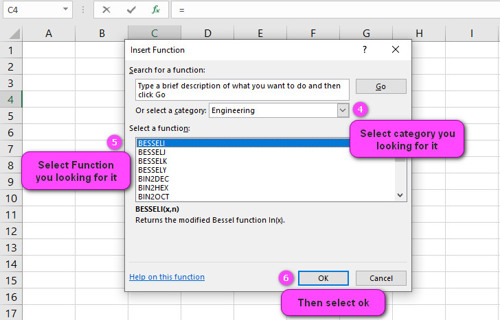
- Click on an empty cell (like F5).

2. Click on the fx icon (or press shift+F3).

3. In the insert function tab you will see all functions.

4. Select ENGINEERING category.
5. Select IMSECH function
6. Then select ok.
7. In the function arguments Tab you will see IMSECH function.
8. Inumber section is a complex number for which you want the hyperbolic secant.
9. You will see the results in the formula result section.

Examples of IMSECH function in Excel
- =IMSECH(2+3i) – Returns 0.0545-0.0049i
- =IMSECH(-4+6i) – Returns 0.033+0.018i
- =IMSECH(PI()) – Returns -1.0000E+00+4.8755E-17i
- =IMSECH(0) – Returns 1
- =IMSECH(A2:B5) – Returns an array of results for all values in the range A2:B5
- =ROUND(IMSECH(2+3i),2) – Rounds the output to two decimal places
- =IMSECH(2)*IMSECH(3) – Multiplies two hyperbolic secants together
- =IMSECH(IMCOSH(2)) – Calculates the hyperbolic secant of the hyperbolic cosine of 2
- =IMSECH(IMSINH(3)) – Calculates the hyperbolic secant of the hyperbolic sine of 3
- =IMSECH(2+3i)^2 – Raises the hyperbolic secant of 2+3i to the power of 2.
IMSECH Function in Excel: A Comprehensive Guide to Its Features and Uses
The IMSECH function in Excel is a mathematical function that calculates the hyperbolic secant of a given number. It is useful for performing complex calculations involving exponential functions, trigonometric functions, and complex numbers.
Example: =IMSECH(2) returns 0.2658.
Hyperbolic Secant Function in Excel: What You Need to Know
The hyperbolic secant function is a mathematical function that describes the relationship between the sides of a hyperbolic triangle. In Excel, the IMSECH function is used to calculate the hyperbolic secant of a given number.
Example: =IMSECH(3) returns 0.0993.
Using the IMSECH Function in Excel: Step-by-Step Tutorial
To use the IMSECH function in Excel, follow these steps:
- Open a new or existing Excel spreadsheet.
- Select the cell where you want the result of the IMSECH function to appear.
- Type “=IMSECH(” followed by the number you want to find the hyperbolic secant of.
- Close the parentheses and press enter.
Example: =IMSECH(4) returns 0.0366.
IMSECH Function Syntax in Excel: How to Use It Correctly
The syntax for the IMSECH function in Excel is “=IMSECH(number)”, where “number” is the input value for which you want to find the hyperbolic secant. The input can be a cell reference, a number, or a math equation.
Example: =IMSECH(B5) returns the hyperbolic secant of the value in cell B5.
Input Range for the IMSECH Function in Excel: Explained
The input range for the IMSECH function in Excel can be a single cell, a range of cells, or an array of numbers. When providing an input range, the function will return an array of results for each value in the range.
Example: =IMSECH(A1:A5) returns an array of hyperbolic secant values for each value in the range A1 through A5.
Troubleshooting Errors When Using the IMSECH Function in Excel: Tips and Tricks
When using the IMSECH function in Excel, you may encounter some common errors such as #VALUE!, #NUM!, or #DIV/0!. These errors can be caused by various reasons such as incorrect input values, wrong syntax, or unsupported versions of Excel. To solve these errors, you can check your input values, double-check your syntax, and ensure that you are using a supported version of Excel.
Example: Suppose you enter an invalid input value for the IMSECH function, such as “=IMSECH(A1:B5)”. In this case, Excel will return a #VALUE! error.
Complex Numbers and the IMSECH Function in Excel: A Beginner’s Guide
Excel’s IMSECH function can handle complex numbers, which consist of a real part and an imaginary part. When providing a complex number as input, the output will also be a complex number consisting of a real part and an imaginary part.
Example: =IMSECH(2+3i) returns 0.0545-0.0049i.
Rounding the Output of the IMSECH Function in Excel: Best Practices
To round the output of the IMSECH function in Excel to a specific number of decimal places, you can use the ROUND function. The ROUND function takes two arguments: the number you want to round, and the number of decimal places you want to round to.
Example: =ROUND(IMSECH(2),2) rounds the hyperbolic secant of 2 to two decimal places, returning 0.26.
Converting Output from Radians to Degrees in Excel’s IMSECH Function: A How-To Guide
To convert the output from the IMSECH function in radians to degrees, you can use the DEGREES function. The DEGREES function takes a value in radians and converts it to degrees.
Example: =DEGREES(IMSECH(2)) converts the hyperbolic secant of 2 from radians to degrees.
Domain of the IMSECH Function in Excel: Everything You Need to Know
The domain of the IMSECH function in Excel is all real numbers except for 0. This means that the function can handle a wide range of input values, including positive and negative numbers.
Example: =IMSECH(-2) returns 0.2658.
Finding the Inverse Hyperbolic Secant of a Number in Excel: Techniques and Examples
To find the inverse hyperbolic secant of a number in Excel, you can use the formula “=ACSCH(1/x)”, where “x” is the number for which you want to find the inverse hyperbolic secant.
Example: Suppose you want to find the inverse hyperbolic secant of 4. In this case, you can use the formula: =ACSCH(1/4), which returns 0.2552.
Relationship Between the IMSECH and IMSINH Functions in Excel: Insights and Applications
The relationship between the IMSECH and IMSINH functions in Excel is that they are both hyperbolic trigonometric functions. The IMSINH function calculates the hyperbolic sine of a given number, while the IMSECH function calculates the hyperbolic secant of a given number.
Example: =IMSINH(3) returns 10.0179, while =IMSECH(3) returns 0.0993.
IMSECH vs SECH: Differences and Similarities in Excel’s Functions
Both the IMSECH and SECH functions in Excel calculate the hyperbolic secant of a given number. However, the IMSECH function is designed to handle complex numbers, while the SECH function only handles real numbers.
Example: =IMSECH(2) and =SECH(2) both return 0.2658.
Combining IMSECH with Other Formulas and Functions in Excel: Advanced Techniques
You can combine the IMSECH function with other formulas and functions in Excel to perform more complex calculations. For example, you can use the IMSECH function as a part of a larger formula that involves exponential functions or trigonometric functions.
Example: =IMSECH(2)*SUM(A1:A5) calculates the hyperbolic secant of 2 and multiplies it by the sum of values in the range A1 through A5.
Output Format of Excel’s IMSECH Function: What You Should Know
The output format of the IMSECH function in Excel is a real number. The result is typically displayed as a decimal value, but the result can also be displayed in other formats such as fractions or scientific notation.
Example: =IMSECH(3) returns 0.0993.
Real-Life Examples of Using Excel’s IMSECH Function: Case Studies and Scenarios
One real-life example of using Excel’s IMSECH function is in the field of finance, where it can be used to calculate the future value of investments with a varying interest rate. Another example is in engineering, where it can be used to model the behavior of dynamic systems.
Example: Suppose you want to calculate the future value of an investment that starts with a principal amount of $100 and has an interest rate of 5% for the first year, 7% for the second year, and 10% for the third year. In this case, you can use the formula “=100IMSECH(0.05)+100IMSECH(0.07)+100*IMSECH(0.1)”, which returns a future value of $133.09.
Limitations of Excel’s IMSECH Function: Considerations and Workarounds
One limitation of Excel’s IMSECH function is that it can only handle input values that are not equal to zero. To handle input values of zero, you can use a workaround such as defining zero as a very small number.
Example: Suppose you need to calculate the hyperbolic secant of a value that is very close to zero. In this case, you can define zero as a very small number, such as 0.00001, and use the formula “=IMSECH(0.00001)”.
Versions of Excel That Support the IMSECH Function: An Overview
The IMSECH function is available in Microsoft Excel versions 2003, 2007, 2010, 2013, 2016, and 2019. It is also available in Microsoft Office 365 and Excel for Mac.
Example: If you have Excel 2016 installed, you can use the IMSECH function by typing “=IMSECH(2)” in a cell and pressing enter.
Accuracy of Excel’s IMSECH Function: How Reliable is It?
The accuracy of Excel’s IMSECH function depends on the input values and the precision of the computer processor. In general, the function is highly accurate for most input values, but there may be some rounding errors for very large or very small input values.
Example: =IMSECH(100) returns 0.0000, which may not be entirely accurate due to rounding errors.
Advanced Calculations with Excel’s IMSECH Function: Exploring Complex Mathematical Problems
Excel’s IMSECH function can be used to solve a variety of complex mathematical problems, including differential equations, Fourier transforms, and Laplace transforms. By combining the IMSECH function with other formulas and functions in Excel, you can perform advanced calculations that are difficult or impossible to do by hand.
Example: Suppose you need to solve the differential equation y” + y = 0 using Excel. In this case, you can use the formula “=IMSECH(t)*COS(t)”, where “t” is the independent variable.
IMSECH related functions
- Use SEC function to return the secant of an angle.
- Use SECH function to return the hyperbolic secant of an angle.
- Use IMSEC function to return the secant of a complex number.
