What is INDEX function in Excel?
The INDEX function is one of the Lookup & reference functions of Excel.
It Returns a value or reference of the cell at the intersection of a particular row and column, in a given range.
We can find this function in Lookup & reference of insert function Tab.
How to use INDEX function in excel
- Click on an empty cell (like F5).

2. Click on the fx icon (or press shift+F3).

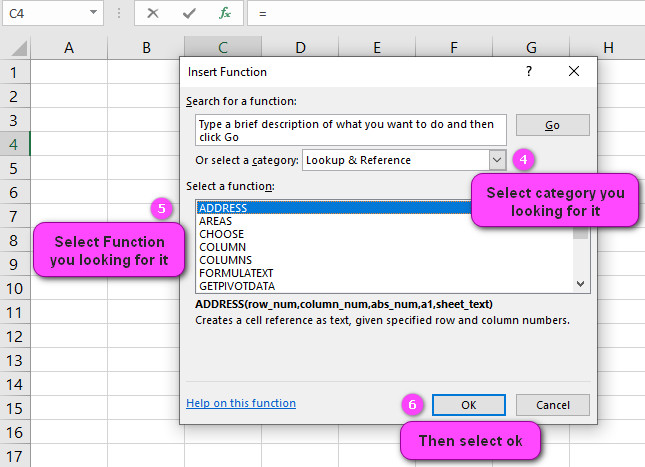
3. In the insert function tab you will see all functions.

4. Select Lookup & reference category.
5. Select INDEX function.
6. Then select ok.
7. In the function arguments Tab, you will see INDEX function.
8. Array Is a range of cells or an array constant.
9. Row_num selects the row in Array or Reference from which to return a value. if omitted, Column_num is required.
10. Column_num selects the Column in Array or Reference from which to return a value. if omitted, Row_num is required.
11. You will see the result in the formula result section.

=INDEX(Table1,2,3) ----->>>>answer is 205Examples of INDEX function in excel
Example 1:
How many ways are to use the INDEX function?
we can use two ways to use index function:
1 . Array form
Returns the value of an element in a table or an array, selected by the row and column number indexes.
Use the array form if the first argument to INDEX is an array constant.

=INDEX({"a","b";"c","d"},2,2) ----->>>>answer is d2 . Reference form
Returns the reference of the cell at the intersection of a particular row and column. If the reference is made up of non-adjacent selections, you can pick the selection to look in.

=INDEX((A2:E5, A7:E10),2,3,2)----->>>>answer is 202Example 2:
What happens If you set row_num or column_num to zero in INDEX function?
If you set row_num or column_num to 0 (zero), INDEX returns the array of values for the entire column or row, respectively. To use values returned as an array, enter the INDEX function as an array formula.

=INDEX(Table1,0,0)----->>>>answer is Table1If you set row_num to 0 (zero), INDEX returns the array of values for the entire column, respectively.

=INDEX(Table1,0,3)----->>>>answer is Column 3If you set column_num to 0 (zero), INDEX returns the array of values for the entire row, respectively.

=INDEX(Table1,2,0)----->>>>answer is Row 2Errors in INDEX function
row_num and column_num must point to a cell within array; otherwise, INDEX returns a #REF! error.

=INDEX(B1,2,2)----->>>>answer is #REF!
Mastering Index Function in Excel: How It Can Boost Your Productivity
Excel is a powerful tool for data analysis and management. One of the most useful functions in Excel is the Index function, which allows you to retrieve specific data points from a table or array quickly and efficiently.
Here’s an example of how to use the Index function in Excel. Suppose you have a table that contains sales data for several products and regions, as shown below:
| Region | Product | Sales |
|---|---|---|
| East | A | 100 |
| East | B | 200 |
| West | A | 150 |
| West | B | 250 |
To extract the sales figure for a specific product and region, you could use the Index function as follows:
- Define named ranges for each column in the table (e.g., “Region”, “Product”, and “Sales”).
- In a separate cell, enter the formula “=Index(Sales,Match(1,(Region=”West”)*(Product=”B”),0))”. This formula retrieves the value in the Sales column where the Region is “West” and the Product is “B”.
- Press Ctrl+Shift+Enter to enter the formula as an array formula.
The formula works by first using the multiplication operator () to create an array of True/False values that match the criteria specified in the formula. For example, the expression “(Region=”West”)(Product=”B”)” evaluates to {0;0;0;1}, which means that the fourth row meets the specified criteria.
The Match function then finds the row number of the True value in the array (i.e., the fourth row). Finally, the Index function retrieves the corresponding value from the Sales column.
By mastering the Index function in Excel, you can become more productive and efficient in your data analysis tasks. With practice and patience, you can develop your skills and become a more effective Excel user.
Everything You Need to Know About Index Function in Excel:
The Index function is a powerful and versatile tool in Microsoft Excel that allows users to retrieve specific data points from a table or array quickly and easily. This function is particularly useful when working with large datasets or when you need to extract specific values from a range of cells.
Syntax: The syntax of the Index function is =INDEX(array,row_num,[column_num]), where “array” is the range of cells containing the data, “row_num” is the row number within the array, and “column_num” (optional) is the column number within the array.
Example: Suppose you have a table of sales data for multiple products and regions, as shown below:
| Region | Product | Sales |
|---|---|---|
| East | A | 100 |
| East | B | 200 |
| West | A | 150 |
| West | B | 250 |
To retrieve the sales figure for a specific product and region, you can use the Index function as follows:
- Define named ranges for each column in the table (e.g., “Region”, “Product”, and “Sales”).
- In a separate cell, enter the formula “=Index(Sales,Match(1,(Region=”West”)*(Product=”B”),0))”. This formula retrieves the value in the Sales column where the Region is “West” and the Product is “B”.
- Press Ctrl+Shift+Enter to enter the formula as an array formula.
In this example, the Match function is used to find the position of the value “1” in an array created by multiplying two logical expressions: “(Region=”West”)” and “(Product=”B”)”. This returns an array of True/False values that match the criteria specified in the formula. The Match function then finds the row number of the True value in the array, which is used as the row number argument in the Index function. Finally, the Index function retrieves the corresponding value from the Sales column.
Top Tips for Using Index Function in Excel Like a Pro:
- Use named ranges to make working with the Index function easier.
- Combine the Index function with other functions like Match, Offset, and Indirect to perform more complex data analysis tasks.
- Take advantage of dynamic arrays to retrieve multiple data points from a table or array in one go.
- Always remember to enter the Index function as an array formula by pressing Ctrl+Shift+Enter.
- Practice using the Index function with different data sets to build your proficiency and confidence.
I hope this helps you understand the power of the Index function in Excel and how it can be used to improve your data analysis workflows.
Expert Insights on Optimizing Index Function in Excel:
The Index function is one of the most powerful tools in Microsoft Excel for data analysis and management. With the right techniques and strategies, users can optimize their use of the Index function to maximize their productivity and efficiency.
Some expert insights on optimizing the Index function in Excel include:
- Use named ranges: Using named ranges can make working with the Index function much easier and more efficient. By creating named ranges for each column in your dataset, you can quickly reference specific ranges of cells in your formulas without having to type out the entire range each time.
- Combine with other functions: The Index function can be combined with other functions like Match, Offset, and Indirect to perform more complex data analysis tasks. By using these functions together, you can create powerful and flexible formulas that allow you to retrieve and manipulate data in new and innovative ways.
- Take advantage of dynamic arrays: Starting from Excel 365, you can use the dynamic array feature to retrieve multiple data points from a table or array in one go. This allows you to simplify your formulas and reduce the number of cells required to achieve your desired results.
- Use array formulas: The Index function is often used as an array formula, which allows you to retrieve multiple values at once. To enter an array formula, select the cell where you want the result to appear, enter the formula, and press Ctrl+Shift+Enter.
Excel Made Easy: Index Function Demystified:
If you’re new to Excel or have never used the Index function before, it can seem intimidating at first. However, with a little practice and guidance, anyone can learn how to use this powerful tool effectively.
To demystify the Index function in Excel, start by understanding its basic syntax and purpose. The Index function retrieves a specific value from a range of cells based on its row and column positions. By specifying the row and column numbers, you can quickly retrieve any value from your dataset without having to manually search for it.
To use the Index function effectively, combine it with other functions like Match, Offset, and Indirect. These functions allow you to perform more complex data analysis tasks and create flexible formulas that adapt to changes in your dataset.
Elevate Your Career with These Index Function Mastery Tips:
As one of the most widely used functions in Excel, mastering the Index function can help elevate your career and improve your productivity. To achieve mastery of this function, follow these tips:
- Practice regularly: Like any skill, mastering the Index function requires practice. Set aside dedicated time each day or week to work on improving your skills and experimenting with new techniques.
- Learn from experts: Take advantage of online resources, books, and courses to learn from Excel experts who have mastered the Index function.
- Experiment with different datasets: By working with a variety of datasets, you can gain a deeper understanding of how the Index function can be used to retrieve and manipulate data to produce meaningful insights.
- Use it in real-world scenarios: Applying the Index function to real-world scenarios is an effective way to reinforce your knowledge and build your confidence in using the function.
The Ultimate Guide to Understanding Index Function in Excel:
The Index function is a powerful and versatile tool in Microsoft Excel that can be used for a wide range of data analysis and management tasks. To understand the Index function fully, start by learning its basic syntax and purpose.
Once you understand how the function works, experiment with different datasets and combine it with other functions to perform more complex data analysis tasks. By following best practices and taking advantage of expert insights, you can master the Index function and elevate your career in Excel.
STREAMLINE YOUR WORKFLOW WITH INDEX FUNCTION IN EXCEL:
The Index function is a powerful tool in Excel that can help to streamline your workflow. By using the Index function, you can easily retrieve specific data points from large datasets, eliminating the need for manual sorting and filtering. Let’s say you have a dataset of sales data that includes columns for date, product name, and total revenue. To retrieve the total revenue for a particular product on a given date, you can use the following formula:
=INDEX(C2:C100,MATCH(1,(A2:A100=”Product A”)*(B2:B100=”01/01/2023″),0))
In this example, we’re using the Match function to find the row number that matches both “Product A” and “01/01/2023”. We then use that row number with the Index function to retrieve the corresponding revenue figure.
SAVE TIME AND INCREASE ACCURACY WITH INDEX FUNCTION IN EXCEL:
Using the Index function in Excel can save you a significant amount of time while also increasing the accuracy of your work. By automating the process of data retrieval, you can eliminate the risk of human error that comes with manual data entry. In addition, the Index function can be used to create dynamic ranges that automatically update as new data is added. For example, if you have a table of sales data that is updated monthly, you can use the following formula to create a dynamic range that always includes the most recent data:
=INDEX(B2:B100,MATCH(MAX(A2:A100),A2:A100,0)):B100
This formula uses the Match function to find the row number that corresponds to the most recent date in column A. We then use that row number to create a dynamic range that starts at that row and continues down to the end of the table.
SIMPLIFYING DATA ANALYSIS WITH INDEX FUNCTION IN EXCEL – A BEGINNER’S GUIDE:
For beginners, the Index function can be an essential tool for simplifying data analysis in Excel. By using the Index function to retrieve specific data points or create dynamic ranges, you can quickly analyze even very large datasets. For example, let’s say you have a table of customer data that includes columns for name, address, and transaction history. You can use the following formula to retrieve the most recent transaction for a particular customer:
=INDEX(C2:C100,MATCH(“John Doe”,A2:A100,0))
In this example, we’re using the Match function to find the row number that corresponds to “John Doe” in column A. We then use that row number with the Index function to retrieve the corresponding transaction data from column C.
ADVANCED STRATEGIES FOR WORKING WITH INDEX FUNCTION IN EXCEL:
For advanced Excel users, there are many strategies for working with the Index function that can help to streamline complex data analysis tasks. One such strategy is to create multi-dimensional arrays using the Index function. For example, if you have a table of sales data that includes columns for date, product name, and revenue, you can use the following formula to create a two-dimensional array that includes both the product names and revenue figures for a given date range:
{INDEX($B2:B100,(MATCH(1,(A2:A100>startDate)∗(A2:2:A100<=endDate),0)))INDEX(C2:2:C100,(MATCH(1,(A2:2:A100>=startDate)∗(A2:2:A$100<=endDate),0)))}
This formula uses the Match function to find the first occurrence of a date within the specified range. We then use two separate Index functions to retrieve the corresponding product name and revenue figures for that date. The curly brackets around the formula indicate that it should be entered as an array formula.
Unlock the Hidden Features of Index Function in Excel
By using the Index function along with other functions like Match and If, you can unlock even more advanced features and capabilities in Excel. For example, you could use it to create dynamic charts and dashboards that update automatically based on user input or changing data.
How to Use Index Function in Excel for Maximum Efficiency
To use the Index function in Excel, you need to provide it with three arguments: the range of cells containing the table, the row number, and the column number. Here’s an example formula:
=INDEX(A1:C3, 2, 3)
This formula retrieves the value in the second row and third column of the range A1:C3.
Advanced Techniques for Mastering Index Function in Excel
One advanced technique for mastering the Index function in Excel is to use it in combination with other formulas to perform complex calculations. For example, you could use the Index function to retrieve data from a large table, then use the Sum or Average function to calculate the total or average of that data.
Another advanced technique is to use the Match function with Index to find specific values within a table. For example, you could use Match to find the row or column number of a particular value, then use Index to retrieve the data in that row or column.
With these advanced techniques and a good understanding of how the Index function works, you can take your Excel skills to the next level and create even more powerful and efficient spreadsheets.
Essential Tips for Taking Your Excel Skills to the Next Level with Index Function
To take your Excel skills to the next level with the Index function, there are a few essential tips to keep in mind:
- Use the Match function with Index to find specific values within a table.
- Use the If function with Index to perform conditional calculations based on certain criteria.
- Use the Offset function with Index to create dynamic ranges and tables that automatically update as new data is added.
By combining these tips with a good understanding of how the Index function works, you can create even more powerful and efficient spreadsheets.
A Beginner-to-Pro Guide to Index Function in Excel
If you’re just starting out with the Index function in Excel, it can seem overwhelming at first. However, with a beginner-to-pro guide, you can quickly learn the basics and start using Index to its full potential.
Here are some key steps to follow when learning the Index function:
- Learn the syntax: The Index function has three arguments – the array, the row number, and the column number. Understanding how to structure the formula correctly is essential.
- Practice retrieving data: Start by practicing retrieving data from a small table or range of cells. Once you’re comfortable with this, move on to larger and more complex tables.
- Explore advanced techniques: Once you’ve mastered the basics, explore advanced techniques like using Index with Match, If, or Offset to perform more complex calculations.
The Benefits of Using Index Function in Excel for Better Data Analysis
Using the Index function in Excel can provide several benefits for better data analysis, including:
- Increased efficiency: By retrieving specific data using Index, you can save time and effort compared to manually searching through a large table.
- More accurate calculations: Using Index with other functions like Match or If can help ensure that your calculations are accurate and based on the right criteria.
- Improved visualization: By using Index to retrieve data for charts and dashboards, you can create more dynamic and interactive visualizations of your data.
By leveraging these benefits, you can improve your data analysis skills and create even more impactful spreadsheets.


