INDIRECT Function in Excel

The INDIRECT function is one of the Lookup & reference functions of Excel.

It returns the reference specified by a text string.

We can find this function in Lookup & reference of insert function Tab.

How to use INDIRECT function in excel

1. Click on empty cell (like F5).

2. Click on fx icon (or press shift+F3).

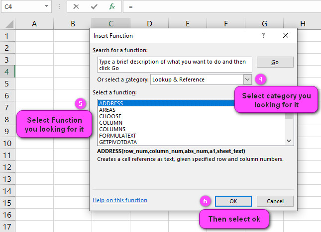
3. In insert function tab you will see all functions.

4. Select Lookup & reference category.

5. Select INDIRECT function.

6. Then select ok

7. In function arguments Tab, you will see INDIRECT function.

8. Ref text is a reference to a cell that contains an A1- or R1 C1-style reference, a name defined as a reference, or a reference to a cell as a text string.

9. A1 is a logical value that specifies the type of reference in Ref text: R1 C1-style= FALSE; A1 style = TRUE or omitted.

10. You will see the result in formula result section.

Examples of INDIRECT function in excel

here are examples of how you can use the INDIRECT function in Excel:

1. Reference a cell based on a text string:
   • =INDIRECT("A1")
     • This will return the value of cell A1.
2. Reference a named range:
   • =INDIRECT("MyRange")
     • This will return the value of the named range “MyRange”.
3. Use a cell reference to dynamically create a range:
   • =INDIRECT("A"&B1)
     • Assuming B1 contains the number 2, this will return the value of cell A2.
4. Create a dynamic range for a chart:
   • =INDIRECT("Sheet1!"&"A1:A"&COUNTA(Sheet1!:A:A))
     • This will create a dynamic range that includes all non-empty cells in column A of Sheet1.
5. Sum a range of cells specified by user input:
   • =SUM(INDIRECT(A1))
     • Assuming A1 contains the text string “B2:C5”, this will sum the values in the range B2:C5.
6. Reference a cell in another workbook:
   • =INDIRECT("[Workbook.xlsx]Sheet1!A1")
     • This will return the value of cell A1 in Sheet1 of Workbook.xlsx.
7. Use a formula to generate the reference:
   • =INDIRECT("A"&MATCH("Search Value",A:A,0))
     • This will return the value of the cell in column A that contains the text string “Search Value”.
8. Create a dropdown list that changes the reference cell:
   • =INDIRECT($A$1)
     • Assuming A1 contains the text string “B2”
9. Reference a worksheet name specified by user input:
   • =INDIRECT("'"&A1&"'!A1") Assuming A1 contains the text string “Sheet1”,
     • this will return the value of cell A1 in Sheet1.
10. Reference a range of cells based on today’s date: =INDIRECT("Sheet1!"&TEXT(TODAY(),"mmddyyyy")&":A10")
    • This will create a dynamic range that starts at the current date in the format “mmddyyyy” and includes all values in column A up to row 10.

Arguments of INDIRECT function in excel

The INDIRECT function in Microsoft Excel takes a text string as input and returns the value of the cell or range of cells specified by that text string.

The syntax of the INDIRECT function is as follows:

=INDIRECT(ref_text, [a1])

The arguments are:

• ref_text:
  • This is the required argument and it specifies the cell reference or range of cells that you want to return.
    • It can be a cell reference (e.g., “A1”) or a named range (e.g., “Sales_Total”).

• a1:
  • This is an optional argument that specifies the format of the returned reference.
    • If a1 is TRUE or omitted, the returned reference is in A1 notation.
    • If a1 is FALSE, the returned reference is in R1C1 notation.

Reference cells in another worksheet by INDIRECT function

the INDIRECT function in Excel can be used to reference cells in another worksheet or workbook.

The syntax for referencing a cell in another worksheet is as follows:

=INDIRECT("SheetName!CellReference")

For example, to reference cell A1 in a worksheet named “Data”, you would use the following formula:

=INDIRECT("Data!A1")

To reference a cell in another workbook, you would use a similar syntax but include the file path and name before the sheet name in the formula. For example:

=INDIRECT("'C:\Users\UserName\Documents[WorkbookName.xlsx]SheetName'!A1")

Note that when referencing cells in other workbooks, you must enclose the entire file path and name in single quotes, and use square brackets around the workbook name.

Create dynamic references by INDIRECT function

The INDIRECT function in Excel can be used to create dynamic references by allowing you to refer to a cell or range of cells using text.

This means that you can create a formula that refers to a cell based on the value in another cell, allowing your formulas to automatically update as your data changes.

Here’s an example of how you can use the INDIRECT function to create a dynamic reference:

Let’s say you have a table of sales data in columns A through C, with the name of each salesperson in column A, the month in column B, and the sales amount in column C.

If you want to create a formula that calculates the total sales for a specific salesperson, you could use the SUMIF function.

However, if you want to make the formula dynamic so that it can calculate the total sales for any salesperson based on a cell reference, you can use the INDIRECT function.

Here are the steps:

1. Start by selecting the cell where you want to display the total sales.
2. In this cell, type the equal sign (=) to start the formula.
3. Type the SUM function, followed by the IF function.
   • The syntax for the SUMIF function is as follows:
     • SUMIF(range, criteria, [sum_range])
       • For this example, the range will be the salesperson names in column A, the criteria will be the name of the salesperson we want to calculate the total sales for, and the sum_range will be the sales amounts in column C.
4. Next, you’ll need to specify the range and criteria arguments for the SUMIF function.
   • To make these arguments dynamic, you can use the INDIRECT function.
5. To do this, first select the cell that contains the name of the salesperson you want to calculate the total sales for.
   • Then copy the cell reference (e.g., A2).
6. Go back to your formula and insert the INDIRECT function into the range argument of the SUMIF function.
   • The syntax for the INDIRECT function is as follows:
     • INDIRECT(ref_text, [a1])
       • In this case, the ref_text argument will be a text string that specifies the cell reference you copied in step 5 (e.g., “A2”).
7. Finally, close the formula with a closing parenthesis and hit enter to calculate the total sales for the selected salesperson.

Your final formula should look something like this:

=SUMIF(INDIRECT(A2&"!A:A"),A3,INDIRECT(A2&"!C:C"))

This formula uses the INDIRECT function to create a dynamic reference to columns A and C of the worksheet specified in the cell reference in cell A2.

The criteria for the SUMIF function are specified in cell A3.

As you change the name of the salesperson in cell A3, the formula will automatically update to calculate the total sales for the selected salesperson.

Errors in INDIRECT function

The INDIRECT function is a useful tool in Excel that allows you to reference cells indirectly. However, there are some potential errors that can occur when using this function.

1. #REF! error:
   • One common error is the #REF! error which occurs when the reference supplied to the INDIRECT function is invalid.
     • This can happen if the referenced cell or range is deleted or moved to another location.
2. #VALUE! error:
   • Another error that can occur is the #VALUE! error which happens when the supplied reference is not a valid text string or a cell reference.
     • For instance, if you provide a numeric value instead of a text string reference, you will get this error.
3. Circular reference error:
   • If the referenced cell or range contains a formula that refers back to the cell containing the INDIRECT function, it can create a circular reference error.
4. Sheet name error:
   • The INDIRECT function can also return an error if the sheet name used in the reference is incorrect or misspelled.

To avoid these errors, you should ensure that the references used in the INDIRECT function are valid and properly formatted.

You can also use functions like ISERROR and IFERROR to handle errors or use alternative approaches such as named ranges or dynamic formulas to achieve the desired results.

INDIRECT function with other Excel functions

INDIRECT function in Excel can be used with other Excel functions.

The INDIRECT function allows you to reference a cell or range of cells indirectly, by referencing a string that contains the cell or range reference as text.

This means that you can use it with other Excel functions that accept cell or range references as arguments.

For example, suppose you have a sheet named “Data” and you want to sum the values in column A for rows 2 to 10.

Instead of manually typing the range reference “Data!A2:A10” into the SUM function, you can use the INDIRECT function to construct the range reference dynamically:

=SUM(INDIRECT("Data!A2:A10"))

In this formula, the string “Data!A2:A10” is passed as an argument to the INDIRECT function, which returns a reference to the range A2:A10 on the “Data” sheet.

The SUM function then calculates the sum of the values in that range.

You can also use the INDIRECT function with other functions that accept cell references as arguments, such as AVERAGEIF, COUNTIF, MAX, MIN, and others.

Just make sure to enclose the cell or range reference inside the INDIRECT function’s parentheses and quotes.

Return a range of cells with INDIRECT function

The INDIRECT function allows you to reference a cell or range of cells indirectly by using a string value that contains the address of the cell or range.

To return a range of cells using the INDIRECT function, you can build a string value that specifies the range of cells you want to reference.

For example, if you want to reference cells A1 through A5, you can build the string value “A1:A5” and use this as the argument for the INDIRECT function.

Here’s an example formula that uses the INDIRECT function to return the sum of values in cells A1 through A5:

=SUM(INDIRECT("A1:A5"))

In this formula, the INDIRECT function returns the range “A1:A5”, which is then used by the SUM function to calculate the total of the values in those cells.

Note that the INDIRECT function can be volatile, meaning that it recalculates every time any change is made to the worksheet.

This can slow down your workbook’s performance, especially if you have many INDIRECT functions in your formulas.

Difference between the INDEX and INDIRECT functions

The INDEX and INDIRECT functions are both used in Microsoft Excel to retrieve data from a specific location within a spreadsheet.

However, there are some important differences between these two functions.

The INDEX function is used to return the value of a cell located at the intersection of a specified row and column in a range or array.

The syntax of the INDEX function is generally as follows:

=INDEX(array,row_num,column_num).

Here, “array” refers to the range or array containing the data you want to retrieve, “row_num” specifies the row number of the cell you want to retrieve, and “column_num” specifies the column number of that cell.

On the other hand, the INDIRECT function is used to return a reference to a cell or range of cells.

The syntax of the INDIRECT function is generally as follows:

=INDIRECT(ref_text,[a1]).

Here, “ref_text” is a string that specifies the cell(s) to which you want to refer, and “[a1]” is an optional argument that specifies whether the cell reference should be interpreted using A1-style or R1C1-style referencing.

In summary, the INDEX function retrieves the value of a specific cell within a range or array, while the INDIRECT function returns a reference to a cell or range of cells.

Combining ADDRESS and INDIRECT functions

There are several ways to combine the INDIRECT and ADDRESS functions in Excel, depending on your specific needs. Here are some examples:

1. Using CONCATENATE

One way to combine INDIRECT and ADDRESS is by using the CONCATENATE function.

You can create a concatenated string that includes the output of the ADDRESS function, and then use the INDIRECT function to return the value in the cell referred to by the concatenation. For example:

=INDIRECT(CONCATENATE("'",Sheet1,"'!",ADDRESS(5,3)))

This formula returns the value in the cell at row 5 and column 3 of Sheet1.

2. Using Ampersand (&)

Instead of using CONCATENATE, you can use the ampersand (&) operator to join text and cell references. The following formula returns the same result as the one above:

=INDIRECT("'"&Sheet1&"'!"&ADDRESS(5,3))

This formula uses the & operator to join the sheet name (in quotes) with the cell reference returned by the ADDRESS function.

3. Nested Formula

You can use nested formulas to combine INDIRECT and ADDRESS.

For example, if you have the sheet name in cell A1, and the row and column numbers in cells B1 and C1, respectively, you can use the following formula:

=INDIRECT("'"&A1&"'!"&ADDRESS(B1,C1))

This formula combines the sheet name, row number, and column number to return the value in the specified cell.

4. Dynamic Range Name

If you want to refer to a range of cells instead of a single cell, you can use a dynamic range name.

For example, if you have a table named Table1 on Sheet1, and you want to sum the values in column B, you can use the following formula:

=SUM(INDIRECT("'"&Sheet1&"'!"&"Table1[Column2]"))

This formula uses the INDIRECT function to create a reference to the range named “Table1[Column2]” on Sheet1.

The SUM function then adds up the values in that range.

Related posts:

Excel ADDRESS Function Most important reason why vlookup not working HYPERLINK Function in Excel FIND Function in Excel