The OFFSET function is one of the Lookup & reference functions of Excel. It returns a
reference to a range that is a given number of rows and columns from a given reference.
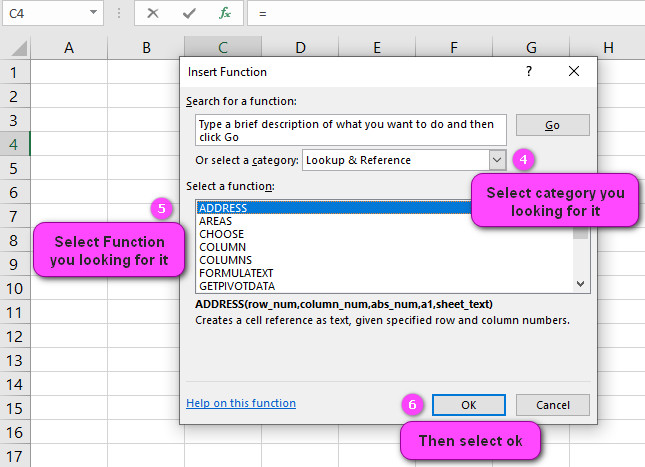
We can find this function in Lookup & reference of insert function Tab.
How to use OFFSET function in excel
- Click on empty cell (like F5).

2. Click on fx icon (or press shift+F3).

3. In insert function tab you will see all functions.

4. Select Lookup & reference category.
5. Select OFFSET function.
6. Then select ok.
7. In function arguments Tab, you will see OFFSET function.
8. Reference is the reference from which you want to base the offset, a reference to a cell or range of adjacent cells.
9. Rows is the number of rows, up or down, that you want the upper-left cell of the result to refer to it.
10. Cols is the number of columns, to the left or right, that you want the upper-left cell of the result to refer to it.
11. Height is the height, in number of rows, that you want the result to be, the same height as Reference if omitted.
12. Width is the width, in number of columns, that you want the result to be, the same width as Reference if omitted.
13. You will see the result in formula result section.
Examples of OFFSET function in excel
Here are a few examples of how to use the OFFSET function in Excel:
- To return a single value: =OFFSET(A2, 1, 2)
This formula returns the value of the cell that is one row down and two columns to the right of cell A2.
- To return a range of values: =OFFSET(B2, 0, 0, 3, 3)
This formula returns a range of values that starts at cell B2 and is three rows tall by three columns wide.
- To create a dynamic named range: =OFFSET(Sheet1!$A1,0,0,COUNTA(Sheet1!1,0,0,COUNTA(Sheet1!A:$A), 4)
This formula creates a dynamic named range that includes all non-blank cells in column A and the next three columns to the right of cell A1 on Sheet1.
These are just a few examples of what you can do with the OFFSET function in Excel.
It’s a powerful tool that can be used in many different ways to manipulate and analyze data.
How do I use the OFFSET function to reference a range of cells?
The OFFSET function in Excel allows you to reference a range of cells that is a specified number of rows and columns away from a starting point.
Here’s how you can use the OFFSET function to reference a range of cells:
- Start by selecting the cell where you want the reference to begin.
- Type “=OFFSET(” into the formula bar.)
- Next, enter the starting cell reference (e.g., A1) followed by a comma.
- Enter the number of rows and columns that you want to move from the starting cell.
- For example, if you want to move three rows down and two columns to the right, you would enter “3, 2” after the starting cell reference.
- Enter the number of rows and columns that you want to include in your range.
- For example, if you want to include a range that is five rows tall and three columns wide, you would enter “5, 3”.
- Close the parentheses and press Enter.
Here’s an example: Let’s say you have a table with data in cells A1:D10, and you want to create a reference to a range of cells that starts in cell B2 and extends three rows down and two columns to the right.
You could use the following formula:
=OFFSET(B2, 3, 2, 3, 2)
This would return a reference to the range of cells C5:D7 (i.e., three rows down and two columns to the right of cell B2, and extending three rows down and two columns to the right).
Can the OFFSET function be used in formulas for dynamic ranges?
Yes, the OFFSET function can be used to create dynamic ranges in Excel formulas. A dynamic range is a range of cells that automatically adjusts its size based on the number of items or rows in a data set.
Here’s an example of how the OFFSET function can be used to create a dynamic range:
Assume you have a table of data in columns A through D, starting at row 1.
You want to create a named range that includes all the data in the table, but you don’t know how many rows there will be.
To create a dynamic named range that includes all the data in the table, you can use the following formula:
=OFFSET($A1,0,0,COUNTA(1,0,0,COUNTA(A:$A),4)
The OFFSET function takes four arguments:
- The starting cell: $A$1
- The number of rows to move down: 0
- The number of columns to move right: 0
- The height of the range: COUNTA(A:A:A)
- The width of the range: 4
The COUNTA function counts the number of non-blank cells in column A, which gives the height of the range.
This means that if you add new rows to the table, the range will automatically expand to include them.
You can name this range by going to Formulas > Define Name and entering a name for the range in the “Name” field.
Now you can use this named range in other formulas throughout your workbook, and it will always refer to the entire table, no matter how many rows it contains.
What are the arguments for the OFFSET function?
Sure! The OFFSET function in Excel takes five arguments:
- Reference: This is the starting cell or range that you want to offset from.
- It can be a range, a reference to a single cell, or a named range.
- Rows: This argument specifies the number of rows to move (up or down) from the reference cell.
- Positive values move down, while negative values move up.
- Columns: This argument specifies the number of columns to move (left or right) from the reference cell.
- Positive values move to the right, while negative values move to the left.
- Height: This argument specifies the height of the range you want to return.
- If this argument is omitted or set to 0, OFFSET returns a reference to a single cell.
- Width: This argument specifies the width of the range you want to return.
- If this argument is omitted or set to 0, OFFSET returns a reference to a single cell.
Here’s an example formula that uses all five arguments:
=OFFSET(A1, 2, 3, 4, 5)
This formula starts at cell A1 and moves down two rows and right three columns.
It then returns a range that is four rows tall and five columns wide.
Note that the size of the range returned by OFFSET depends on the values of the last two arguments (height and width).
By changing these arguments or omitting them entirely, you can use OFFSET to return a single cell, a row, a column, or a larger range of cells.
It’s worth noting that the OFFSET function can be volatile, meaning it recalculates every time any change is made to the worksheet.
This can slow down your workbook if used excessively or in large data sets.
Can the OFFSET function be used to create a named range?
Yes, the OFFSET function can be used to create a named range in Excel.
A named range is a user-defined name that refers to a specific range of cells in a worksheet.
To create a named range using OFFSET, you can follow these steps:
- Select the cell or range of cells that you want to name.
- Click on the “Formulas” tab in the ribbon.
- Click on the “Define Name” button. This will open the “New Name” dialog box.
- In the “Name” field, enter a unique name for the range.
- In the “Refers to” field, enter the OFFSET formula with the appropriate arguments.
For example, let’s say you have a table in columns A through D, starting at row 2.
You want to create a named range called “MyTable” that includes all the data in the table, but you don’t know how many rows there will be.
You can use the following formula:
=OFFSET($A2,0,0,COUNTA(2,0,0,COUNTA(A:A)−1,COLUMNS(A)−1,COLUMNS(A:D))
The OFFSET function takes five arguments, as follows:
- The starting cell: $A$2
- The number of rows to move down: 0
- The number of columns to move right: 0
- The height of the range: COUNTA(A:A:A)-1 (to exclude the header row)
- The width of the range: COLUMNS($A:D) (to include all four columns)
This formula creates a named range called “MyTable” that includes all the data in the table.
Note that the COUNTA function counts the number of non-blank cells in column A, which gives the height of the range, and the COLUMNS function returns the number of columns in the range.
Once you’ve created a named range, you can refer to it in formulas and other parts of your workbook by its name, rather than by its cell references.
This can make your formulas easier to read and maintain.
How do I use the OFFSET function to return a value from a specific cell?
Sure, here’s an explanation on how to use the OFFSET function to return a value from a specific cell in Excel.
The OFFSET function can be used to return a value from any cell that is a specified number of rows and/or columns away from a starting cell.
To use the OFFSET function to return a value from a specific cell, you just need to provide the correct arguments to the function.
Here’s an example formula that uses the OFFSET function to return a value from a specific cell:
=OFFSET(A1, 2, 3)
In this formula, “A1” is the starting cell, “2” is the number of rows to move down, and “3” is the number of columns to move right.
This formula returns the value of the cell that is two rows down and three columns to the right of A1.
You can modify this formula to refer to a different starting cell or to move a different number of rows and columns.
For example, if you wanted to return the value of the cell that is one row above and two columns to the left of cell D5, you could use the following formula:
=OFFSET(D5, -1, -2)
In this formula, “D5” is the starting cell, “-1” is the number of rows to move up, and “-2” is the number of columns to move left.
This formula returns the value of the cell that is one row above and two columns to the left of D5.
Note that the OFFSET function can also be used to return a range of cells instead of a single value.
To do this, you just need to specify the height and width of the range using additional arguments in the OFFSET function.
How do I use the OFFSET function to return a range of values?
To use the OFFSET function to return a range of values, you just need to include two additional arguments in the formula to specify the height and width of the range.
Here’s an example formula that uses the OFFSET function to return a range of values:
=OFFSET(A1, 2, 3, 4, 2)
In this formula, “A1” is the starting cell, “2” is the number of rows to move down, “3” is the number of columns to move right, “4” is the height of the range, and “2” is the width of the range.
This formula returns a range of values that starts two rows down and three columns to the right of A1 and is four rows tall by two columns wide.
You can modify this formula to return a different range of values by changing the starting cell, the number of rows and/or columns to move, and/or the height and width of the range.
For example, let’s say you have a table of data in columns A through D, starting at row 2.
You want to create a formula that returns the average of the values in the second column of the table.
You can use the following formula:
=AVERAGE(OFFSET($B2,0,0,COUNTA(2,0,0,COUNTA(A:$A)-1, 1))
In this formula, “B2” is the starting cell for the range, “0” is the number of rows to move down, “0” is the number of columns to move right, “COUNTA(A:A:A)-1” is the height of the range (to exclude the header row), and “1” is the width of the range (to include only the second column).
This formula creates a range that starts at cell B2 and extends down the entire height of the table, but includes only the second column.
The AVERAGE function then calculates the average of the values in this range.
Note that you can use any function that operates on a range of values with the OFFSET function to return a range of results.
Can the OFFSET function be used with other functions, such as SUM, AVERAGE, or COUNT?
Yes, the OFFSET function can be used with other functions such as SUM, AVERAGE, or COUNT to perform calculations on a range of values specified by the OFFSET function.
Here’s an example using the SUM function:
Let’s say you have a table of data in columns A through D, starting at row 2.
You want to create a formula that sums the values in the third column of the table. You can use the following formula:
=SUM(OFFSET($C$2,0,0,COUNTA($A:$A)-1,1))
In this formula, “C2” is the starting cell for the range, “0” is the number of rows to move down, “0” is the number of columns to move right, “COUNTA(A:A:A)-1” is the height of the range (to exclude the header row), and “1” is the width of the range (to include only the third column).
This formula creates a range that starts at cell C2 and extends down the entire height of the table, but includes only the third column.
The SUM function then calculates the sum of the values in this range.
Similarly, you can use other functions like AVERAGE or COUNT with the OFFSET function, depending on your needs.
Here’s another example using the AVERAGE function:
=AVERAGE(OFFSET(A1,2,0,5,1))
In this formula, “A1” is the starting cell for the range, “2” is the number of rows to move down, “0” is the number of columns to move right, “5” is the height of the range, and “1” is the width of the range.
This formula creates a range that starts two rows down from cell A1 and is five rows tall by one column wide.
The AVERAGE function then calculates the average of the values in this range.
Overall, using the OFFSET function with other functions can be a powerful way to perform calculations on specific ranges of data in your workbook.
How can I use the OFFSET function to create a scrolling chart in Excel?
You can use the OFFSET function in Excel to create a scrolling chart that displays a specific number of data points at a time.
This can be useful for visualizing trends or patterns in a large data set.
Here’s an example of how you can create a scrolling chart using the OFFSET function:
- First, create a table of data with your values and corresponding dates. For example:
| Date | Value |
|---|---|
| 01/01/2022 | 10 |
| 02/01/2022 | 15 |
| 03/01/2022 | 23 |
| 04/01/2022 | 27 |
| 05/01/2022 | 30 |
| … | … |
- Create a line chart with your entire data set, including all dates and values.
- Add two spin buttons to your worksheet by going to Developer > Insert > Spin Button. Place them next to your chart.
- Right-click on one of the spin buttons and choose “Format Control”.
- In the “Input Range” field, enter a cell where you want the spin button value to be stored (e.g., cell A1).
- In the “Minimum Value” and “Maximum Value” fields, enter the minimum and maximum values for the spin button (e.g., 1 and the total number of data points).
- In the “Input Range” field, enter a cell where you want the spin button value to be stored (e.g., cell A1).
- Repeat step 4 for the other spin button, using a different cell to store its value (e.g., cell B1).
- Now, create a named range called “DataRange” that includes only the data points that you want to show on the chart.
- You can use the OFFSET function to create this dynamic range based on the values of the spin buttons.
For example, if you want to show 10 data points at a time, you can use the following formula:
=OFFSET($B$2,A1-1,0,10,1)
In this formula, “B2” is the starting cell for the range, “A1-1” is the number of rows to move down (based on the value of the first spin button), “0” is the number of columns to move right, “10” is the height of the range (to show 10 data points at a time), and “1” is the width of the range (to include only the second column).
- Finally, update your chart’s data source to use the named range “DataRange” instead of the original data range.
Now, when you click on the spin buttons, the chart will scroll to display the next set of data points based on the values of the spin buttons.
Overall, using the OFFSET function in combination with spin buttons and a named range can allow you to create a powerful scrolling chart that displays a specific number of data points at a time.
Are there any limitations or drawbacks to using the OFFSET function?
Yes, there are some limitations and drawbacks to using the OFFSET function in Excel.
- Volatility: The OFFSET function is considered volatile, which means that it will recalculate every time any change is made to the worksheet, even if the change has no effect on the formula’s result.
- This can slow down your workbook if used excessively or with large data sets.
- Error-prone: If the arguments to the OFFSET function are not entered correctly, it can return unexpected results or errors.
- For example, if you specify a negative value for the “height” argument, the function may return a reference to a cell outside the range of data.
- It’s important to double-check your formulas when using OFFSET to avoid these issues.
- Limited functionality: While the OFFSET function is useful for creating dynamic ranges and scrolling charts, it has some limitations in terms of functionality.
- For example, it cannot be used with structured references or tables, and it cannot refer to cells on other worksheets or workbooks.
- Compatibility issues: The OFFSET function may not be compatible with older versions of Excel, particularly those prior to Excel 2007.
- If you need to share your workbook with others, you should check to ensure that they are using a version of Excel that supports the function.
- Performance issues: If you use the OFFSET function in combination with other functions that perform calculations on large data sets, such as SUM or AVERAGE, it can slow down the performance of your workbook.
- To mitigate this issue, you can consider using alternative functions like INDEX and MATCH or dynamic named ranges.
Despite these limitations and drawbacks, the OFFSET function can still be a powerful tool for creating dynamic ranges and scrolling charts in Excel.
It’s important to use the function judiciously and double-check your formulas to avoid errors or unexpected results.

