What is ROW function in Excel?
The ROW function is one of the Excel Lookup & reference functions.
It returns the ROW number of a reference.
We can find this function in Lookup & reference of insert function Tab.
How to use row function in excel
- Click on empty cell (like F5 )

2. Click on the fx icon (or press shift+F3)

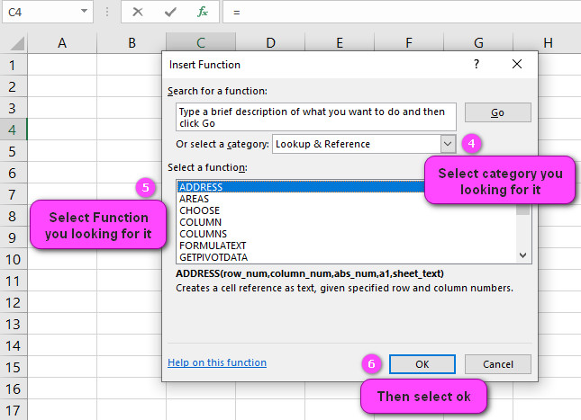
3. In the insert function tab you will see all functions

4. Select Lookup & reference category
5. Select ROW function
6. Then select ok
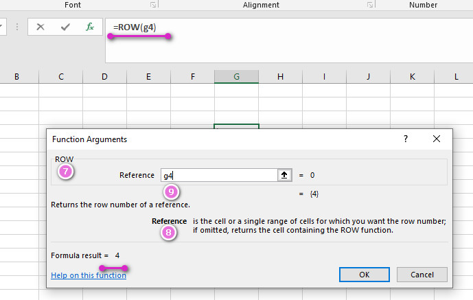
7. In the function arguments Tab, you will see ROW function
8. In the Reference section you can enter the cell or a single range of cells that you want the ROW number.
9. If you click on G4, see result 4
10. If you click on A2, see result 2
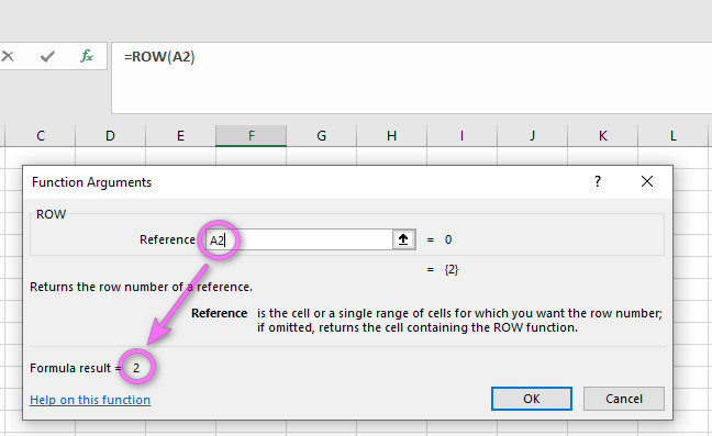
11. You will see the result in formula result section
Examples of ROW function in excel
Examples of row functions in Excel:
- ROW(): Returns the row number of a selected cell. For example, =ROW(A1) returns 1.
- ROWS(): Counts the number of rows in a range of cells. For example, =ROWS(A1:A5) returns 5.
- ROWS and IF: Returns the number of rows that contain data. For example, =IF(ROWS(A1:A5)>0, “There is data in the range”, “The range is empty”).
- ROWS and INDIRECT: Uses the INDIRECT function to count the number of rows in a named range. For example, =ROWS(INDIRECT(“MyNamedRange”)).
- ROWS and INDEX: Uses the INDEX function to count the number of rows in an array. For example, =ROWS(INDEX(A1:C10,1,0)) returns 10.
- ROWS and MATCH: Uses the MATCH function to count the number of rows in a column that match a specific criteria. For example, =ROWS(MATCH(“Apple”,A1:A10,0)) returns the number of rows that contain the word “Apple”.
- ROWS and OFFSET: Uses the OFFSET function to count the number of rows in a range that starts from a particular cell. For example, =ROWS(OFFSET(A1,0,0,5,1)) returns 5.
- ROWS and SUMPRODUCT: Uses the SUMPRODUCT function to count the number of non-empty cells in a range. For example, =SUMPRODUCT(–(A1:A10<>””)) returns the number of non-empty cells in the range A1:A10.
- ROWS and COUNTIF: Uses the COUNTIF function to count the number of cells in a range that meet a specific criteria. For example, =ROWS(COUNTIF(A1:A10,”>50″)) returns the number of cells in the range A1:A10 that contain a value greater than 50.
- ROWS and MAX: Uses the MAX function to return the maximum row number for a selected range of cells. For example, =MAX(ROW(A1:A10)) returns 10.
Example 1: How to Automatic row numbering in the Excel
We can use ROW function if we want to number a set of data in Excel.
First, suppose we have data as shown in the image below:
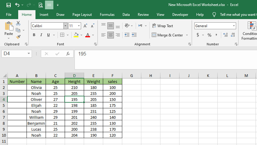
We can automatically number cells 2 to 10 by the ROW function, By Typing =ROW()-1 in cells.

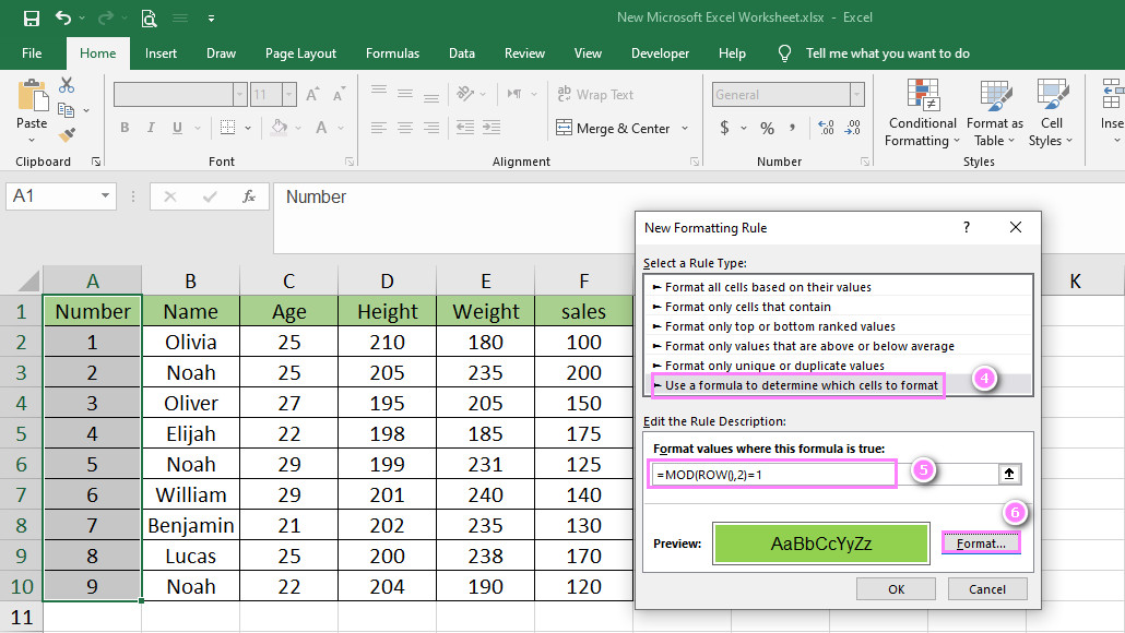
Example 2: How to Highlight Every other Row in the Excel
If we want Highlight Every other Row in Excel, we can combine ROW, MOD and Conditional formatting:
1. Select column A
2. In Home Tab, Choose Conditional formatting.(Press ALT+H+L)
3. Select New Rule. (Press ALT+H+L+N)

4. In New Formatting Rule Tab, Select Use a Formula to determine Which Cells To Format.
5. In formula box, Type =MOD(ROW(),2)=1
6. Select Format
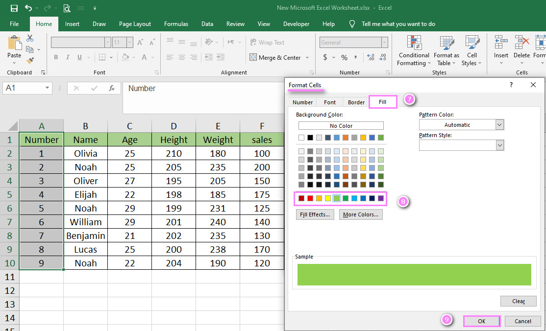
7. In the Format cell Tab, Select Fill.
8. In Fill Tab, Select your Color.
9. Finally Select ok.
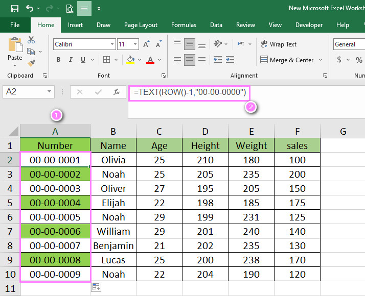
Example 3: HOW to Generate Specific Serial Number in Excel
If we want Generate Specific Sequential Serial numbers in Excel, we can combine ROW and Text:
1. Choose your format text (ex: “00-00-0000”)
2. Type in cell A2 =TEXT(ROW(A2)-1,”00-00-0000″)
3. Drag the fill handle to the last cell of the range.
Things to Remember
- The argument of this function is required and not optional
- If a reference is omitted, the cell containing the ROW function is used.
- This function is available for all excel versions(2007-2019)
Python code for ROW function
| Name | Age | Height | Weight |
| Olivia | 25 | 210 | 180 |
| Noah | 25 | 205 | 235 |
| Oliver | 27 | 195 | 205 |
| Elijah | 22 | 198 | 185 |
| James | 29 | 199 | 231 |
| William | 29 | 201 | 240 |
| Benjamin | 21 | 202 | 235 |
| Lucas | 25 | 200 | 238 |
| Henry | 22 | 204 | 190 |
import pandas as pd

df=pd.read_csv(‘example.csv’)

maxrow=df['Name'].notna().sum()

print (maxrow)
Discovering the Power of the ROW Function in Excel
The ROW function in Excel is used to return the row number of a given cell. However, it can also be used creatively to perform various other operations, such as generating a series of sequential numbers or creating dynamic references to cells. An example of this might be using the ROW function with the INDIRECT function to reference different cells based on their relative position to a starting point.
Get to Know the Syntax of the ROW Function in Excel
The syntax of the ROW function is simply “=ROW(cell_reference)” where “cell_reference” is the reference to the cell you want to return the row number for. For example, if you wanted to find out what row number cell A1 was in, you would enter “=ROW(A1)” in a different cell and it would return the value 1.
Learn How to Use the ROW Function to Return the Row Number of a Cell
This is a basic but crucial function for many Excel tasks, especially when dealing with larger spreadsheets. As mentioned above, the syntax for using the ROW function to return the row number of a cell is simply “=ROW(cell_reference)”. For example, if you wanted to find out what row number cell F20 was in, you would enter “=ROW(F20)” in a different cell and it would return the value 20.
Mastering the Use of the ROW Function with Multiple Cells and Ranges
This can be useful for a variety of tasks, such as referencing a range of cells that starts at a certain row number or performing calculations based on the row numbers of different cells. To use the ROW function with multiple cells or ranges, you can simply use an array formula. For example, if you wanted to find the row numbers for cells A1:A5, you would enter “{=ROW(A1:A5)}” in a different cell and it would return an array of row numbers (1, 2, 3, 4, 5). Note that array formulas must be entered by pressing Ctrl+Shift+Enter, not just Enter.
Using Relative and Absolute References with the ROW Function in Excel
Using relative references means that when you copy a formula containing the ROW function to another cell, the reference will change relative to where it is copied. Absolute references, on the other hand, will remain constant regardless of where the formula is copied. An example of this would be using absolute referencing with the ROW function to always reference the first row of a range, such as “$A$1:ROW(A1)”.
Revolutionize Your Conditional Formatting with the ROW Function in Excel
Conditional formatting allows you to automatically format cells based on certain rules or criteria. By using the ROW function within conditional formatting, you can apply different formatting to different rows or sets of rows. An example of this might be highlighting every other row by using the formula “=MOD(ROW(),2)=0” in the conditional formatting rule.
Maximizing the Efficiency of Other Functions with the ROW Function in Excel
One way to do this is by using the ROW function within an INDEX or MATCH function to create dynamic references to specific cells based on their position relative to other cells. Another example might be using the ROW function with the OFFSET function to dynamically return a range of data based on a given starting point.
Creating Dynamic Formulas with the ROW Function in Excel
Dynamic formulas are formulas that adjust automatically based on changing data, which can save a lot of time and effort in larger spreadsheets. One example of using the ROW function to create dynamic formulas would be using it within a VLOOKUP function to return values from a table that may change in size or location over time.
Streamlining Data Filtering and Sorting with the ROW Function in Excel
By using the ROW function to create indexes for your data, you can easily sort and filter your data based on specific criteria. For example, you could add a column next to your data and use the ROW function to populate it with index numbers, then easily sort your data by this index column.
Generating Number Series with Ease Using the ROW Function in Excel
The ROW function can be used to generate a series of sequential numbers simply by copying and pasting the formula down a column. An example of this might be using the formula “=ROW()-1” to generate a series of numbers starting at zero (0, 1, 2, 3, etc.).
Creating Unique Identifiers for Each Row with the ROW Function in Excel
This title implies that the article will teach the reader how to use the ROW function in Excel to create unique identifiers for each row of data. This can be useful when working with large datasets or when merging data from different sources. One example of this would be using the ROW function within a CONCATENATE function to create a unique identifier that combines the contents of different cells along with the row number.
Taking Your Lookup Functions to the Next Level with the ROW Function in Excel
By using the ROW function to dynamically reference different cells or ranges, you can create more advanced lookup functions that can handle changing data. An example of this might be using the ROW function within an INDEX or MATCH function to return a value from a table that is offset by a certain number of rows based on the result of another formula or function.
Create Easy-to-Use Tables of Contents with the ROW Function in Excel
By using the ROW function to reference different cells or ranges, you can dynamically create links to different parts of your spreadsheet. An example of this might be using the HYPERLINK function in combination with the ROW function to create clickable links that take the user to specific sections of the spreadsheet.
Efficiently Deleting Rows in Excel with the ROW Function
By using the ROW function within a formula that identifies which rows to delete, you can quickly and easily remove unwanted data from your spreadsheet. An example of this might be using the formula “=IF(ROW()<5,”Delete”,”Keep”)” to mark all rows below the fourth row for deletion.
Combining the Power of INDEX, MATCH, and the ROW Function in Excel
By using the ROW function to dynamically reference different cells or ranges, you can make your lookup formulas more flexible and adaptable to changing data. An example of this might be using the ROW function within the MATCH function to return the row number of a specific value, then using the INDEX function to return a value from a different column in the same row.
Calculating Percentages with the Versatile ROW Function in Excel
The ROW function can be used to create dynamic references to specific cells or ranges, which can be useful for calculating percentages based on changing data. An example of this might be using the ROW function within a formula that calculates the percentage of total sales for each product in a table, where the denominator of the percentage calculation is the sum of all sales values in the table.
Counting Rows Made Easy with the ROW Function in Excel
By using the ROW function within a formula that counts the number of rows in a given range, you can automate the row counting process and avoid manual errors. An example of this might be using the formula “=ROWS(A1:A10)” to count the number of rows in a range of cells.
Inserting Blank Rows into Worksheets with the ROW Function in Excel
By using the ROW function within a formula that identifies where to insert new rows, you can automate the process of adding space between existing rows. An example of this might be using the formula “=IF(MOD(ROW(),2)=0,””,”Insert Row Here”)” to identify every other row for a new blank row insertion.
Highlighting Specific Rows in Excel with the ROW Function
By using the ROW function within a formula that identifies which rows to highlight, you can draw attention to important or relevant data in your worksheet. An example of this might be using the formula “=IF(MOD(ROW(),2)=0,TRUE,FALSE)” to highlight every other row of data with a different color or formatting.
Visualizing Data with Charts and Graphs Using the ROW Function in Excel
By using the ROW function within a formula that references data in a table or range, you can create dynamic charts and graphs that update automatically as your data changes. An example of this might be using the ROW function within a formula that creates a line graph showing the trend of sales over time, where each row represents a different time period.
ROW related functions :
- Column function
- Indirect function
- Offset function
- SMALL function


