The SORT function is one of the Lookup & reference functions of Excel.
It looks up a value either from a one-row or one-column range or from an array. Provided for backward compatibility.
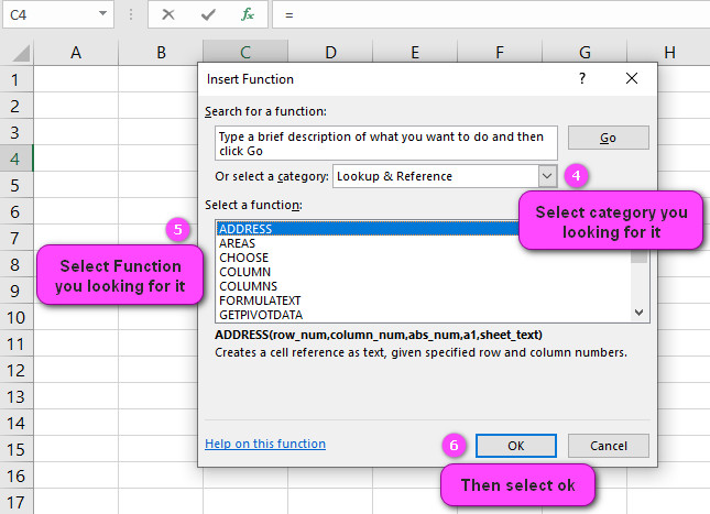
We can find this function in Lookup & reference of insert function Tab.
How to use SORT function in excel
- Click on empty cell (like F5).

2. Click on fx on the below of font word (or press shift+F3)

3. In insert function tab you will see all functions

4. Select Lookup & reference category
5. Select SORT function
6. Then select ok
7. In function arguments Tab, you will see SORT function
8. Lookup value is a value that SORT searches for in Lookup vector and can be a number,
text, a logical value, or a name or reference to a value
9. Lookup vector is a range that contains only one row or one column of text, numbers, or
logical values, placed in ascending order
10. Result vector is a range that contains only one row or column, the same size as lookup vector
11. Lookup value is a value that LOOKUP searches for in Array and can be a number, text, a
logical value, or a name or reference to a value
12. Array is a range of cells that contain text, number, or logical values that you want to
compare with Lookup value
13. You will see the result in formula result section
Examples of SORT function in excel
Here are some examples of how to use the SORT function in Excel:
Example 1: Sort a column of numbers in ascending order
Assuming you have a column of numbers in A1:A5, you can sort them in ascending order using the SORT function as follows:
=SORT(A1:A5)
This will return a new array with the same numbers, but sorted in ascending order.
Example 2: Sort a range of values by multiple columns
Assuming you have a table of data with headers in A1:C5, where column A contains names, column B contains salaries, and column C contains years of service, you can sort the table first by salary in descending order, and then by name in ascending order using the SORT function as follows:
=SORT(A1:C5, 2, -1, 1, 1)
This will return a new array with the same data, but sorted first by salary in descending order, and then by name in ascending order.
Example 3: Sort a range of values using a custom sort order
Assuming you have a column of text values in A1:A5, and you want to sort them according to a custom order (e.g., “High”, “Medium”, “Low”), you can use the SORT function with a custom list as follows:
=SORT(A1:A5, , , {"Low","Medium","High"})
This will return a new array with the same text values, but sorted according to the custom order specified.
Example 4: Sort a range of values by date
Assuming you have a column of dates in A1:A5, you can sort them in ascending order using the SORT function as follows:
=SORT(A1:A5, 1, 1)
This will return a new array with the same dates, but sorted in ascending order.
Note that the SORT function can also be combined with other functions or formulas to create more complex sorting criteria.
For example, you could use CONCATENATE function to combine values from multiple columns into a single key for sorting.
How do I sort data in Excel using the SORT function?
how to sort data in Excel using the Sort function, step-by-step:
Step 1: Select the range of cells that you want to sort, including any headers or labels that you want to keep with their respective columns.
For example, if you have a table with sales data that includes column headers (like “Region”, “Product”, and “Sales”), select all of the data including the headers.
Step 2: Click on the “Data” tab in the ribbon at the top of the Excel window.
Step 3: In the “Sort & Filter” group, click on the “Sort” button. This will open the “Sort” dialog box.
Step 4: In the “Sort” dialog box, you can choose how you want to sort your data.
For example, you can sort by one or more columns, in ascending or descending order, and even add additional sorting criteria.
Let’s say we want to sort our sales data by Region first (in alphabetical order), and then by Sales (in descending order).
Step 5: In the “Sort” dialog box, under “Column”, select the column you want to sort by first. In this case, we’ll select “Region”.
Step 6: Under “Sort On”, choose how you want to sort the data. You can sort by cell color, font color, values, and more. For now, let’s stick with sorting by values.
Step 7: Under “Order”, choose whether you want to sort in ascending or descending order. We’ll choose “A to Z” for Region.
Step 8: If you want to add additional sorting criteria, click on the “Add Level” button and repeat steps 5-7 for each level of sorting you want to apply.
Step 9: Once you’re finished setting up your sorting options, click on the “OK” button. Excel will sort your data based on the criteria you specified.
Here’s an example of what our sales data table might look like before and after sorting:
Before Sorting:
| Region | Product | Sales |
|---|---|---|
| North America | Widget A | $10,000 |
| Europe | Widget B | $5,000 |
| Asia | Widget C | $2,500 |
| North America | Widget D | $15,000 |
| Europe | Widget E | $7 |
What are the different options available for SORTING data in Excel?
Sure!
Excel offers several different options for sorting data, including:
- Sort by values: This is the most common way to sort data in Excel.
- When you sort by values, Excel will sort your data based on the numerical or alphabetical values in each cell.
For example, if you have a column of numbers ranging from 1 to 10, sorting by values in ascending order would put the number 1 at the top of the column and the number 10 at the bottom.
- Sort by cell color or font color: If you’ve formatted your cells with different colors, you can sort them based on those colors.
- For example, you might want to sort a table of tasks based on priority, where high-priority tasks are highlighted in red and low-priority tasks are highlighted in green.
- Sort by cell icon: Excel also allows you to sort data based on cell icons, which can be useful if you’re using conditional formatting to highlight certain cells based on specific criteria.
For example, if you’re tracking project progress with a Gantt chart, you might use arrows to indicate whether each task is ahead of or behind schedule.
You could then sort your data based on those arrows to quickly see which tasks are falling behind.
- Sort by custom list: If you have a specific order in mind for your data (for example, if you’re sorting a list of months or days of the week), you can create a custom list and sort your data based on that list.
- Sort by cell value length: Excel also allows you to sort data based on the length of the text in each cell.
- This can be useful if you’re working with text strings of varying lengths and want to sort them based on how long they are.
These are just a few examples of the different sorting options available in Excel.
To access these options, simply click on the “Sort” button in the “Data” tab and choose the option that best fits your needs.
Can I SORT multiple columns at once in Excel?
How to sort multiple columns at once in Excel
Step 1: Select the range of cells that you want to sort, including any headers or labels that you want to keep with their respective columns.
Step 2: Click on the “Data” tab in the ribbon at the top of the Excel window.
Step 3: In the “Sort & Filter” group, click on the “Sort” button. This will open the “Sort” dialog box.
Step 4: In the “Sort” dialog box, you can choose how you want to sort your data.
For example, you can sort by one or more columns, in ascending or descending order, and even add additional sorting criteria.
Step 5: To sort multiple columns, click on the “Add Level” button in the “Sort” dialog box.
This will add another level of sorting criteria.
Step 6: Choose the column you want to sort by next, and set your sorting options as desired.
For example, you might sort by Region first, then by Product.
Step 7: If you want to add additional levels of sorting, click on the “Add Level” button again and repeat steps 6 and 7 for each level of sorting you want to apply.
Step 8: Once you’re finished setting up your sorting options, click on the “OK” button.
Excel will sort your data based on the criteria you specified.
Here’s an example of what a table might look like before and after sorting multiple columns:
Before Sorting:
| Region | Product | Sales |
|---|---|---|
| North America | Widget A | $10,000 |
| Europe | Widget B | $5,000 |
| Asia | Widget C | $2,500 |
| North America | Widget D | $15,000 |
| Europe | Widget E | $7,500 |
| Asia | Widget F | $3,750 |
After Sorting by Region (A to Z) and then by Sales (largest to smallest):
| Region | Product | Sales |
|---|---|---|
| Asia | Widget C | $2,500 |
| Asia | Widget F | $3,750 |
| Europe | Widget E | $7,500 |
| Europe | Widget B | $5,000 |
| North America | Widget D | $15,000 |
| North America | Widget A | $10,000 |
In this example, we sorted the data first by Region in alphabetical order (A to Z), and then within each region, we sorted by Sales in descending order (largest to smallest).
What is the difference between sorting by values and sorting by cell color or font color?
Sorting by values and sorting by cell color or font color are two different ways to sort data in Excel.
Sorting by values means that Excel will look at the numerical or alphabetical values in each cell and sort them accordingly.
For example, if you have a column of numbers ranging from 1 to 10, sorting by values in ascending order would put the number 1 at the top of the column and the number 10 at the bottom.
On the other hand, sorting by cell color or font color means that Excel will look at the formatting of each cell and sort them based on the color of the cell or font.
This can be useful if you’re using color-coding to highlight specific cells or rows based on certain criteria.
For example, let’s say you have a table of tasks with columns for Task Name, Start Date, End Date, and Status.
You use conditional formatting to highlight tasks that are behind schedule in red, tasks that are on track in yellow, and tasks that are ahead of schedule in green.
If you want to quickly see all of the tasks that are behind schedule, you can sort the table by cell color and Excel will bring all of the red cells to the top of the table.
Here’s an example of what a table might look like before and after sorting by cell color:
Before Sorting:
| Task Name | Start Date | End Date | Status |
|---|---|---|---|
| Task 1 | 1/1/2022 | 1/15/2022 | On Track |
| Task 2 | 1/5/2022 | 1/20/2022 | Behind |
| Task 3 | 1/10/2022 | 1/30/2022 | Ahead |
| Task 4 | 1/15/2022 | 2/1/2022 | Behind |
| Task 5 | 1/20/2022 | 2/15/2022 | On Track |
After Sorting by Cell Color:
| Task Name | Start Date | End Date | Status |
|---|---|---|---|
| Task 2 | 1/5/2022 | 1/20/2022 | Behind |
| Task 4 | 1/15/2022 | 2/1/2022 | Behind |
| Task 1 | 1/1/2022 | 1/15/2022 | On Track |
| Task 5 | 1/20/2022 | 2/15/2022 | On Track |
| Task 3 | 1/10/2022 | 1/30/2022 | Ahead |
In this example, we sorted the table by cell color in ascending order, which brought all of the red (behind schedule) cells to the top of the table.
How do I SORT data in descending order in Excel?
Sure! Sorting data in descending order in Excel is very similar to sorting it in ascending order.
Here’s how you can sort data in descending order:
Step 1: Select the range of cells that you want to sort, including any headers or labels that you want to keep with their respective columns.
Step 2: Click on the “Data” tab in the ribbon at the top of the Excel window.
Step 3: In the “Sort & Filter” group, click on the “Sort” button. This will open the “Sort” dialog box.
Step 4: In the “Sort” dialog box, choose the column or columns that you want to sort by.
Step 5: Under “Order”, choose “Z to A” for text data or “Largest to Smallest” for numerical data. This will tell Excel to sort your data in descending order.
Step 6: If you want to sort by multiple columns, you can add additional levels of sorting as needed. Just click on the “Add Level” button and repeat steps 4 and 5 for each level of sorting.
Step 7: Once you’re finished setting up your sorting options, click on the “OK” button. Excel will sort your data based on the criteria you specified.
Here’s an example of what a table might look like before and after sorting in descending order:
Before Sorting:
| Name | Age | Gender |
|---|---|---|
| Alice | 25 | Female |
| Bob | 30 | Male |
| Charlie | 27 | Male |
| Dave | 22 | Male |
| Emily | 28 | Female |
After Sorting by Age in Descending Order:
| Name | Age | Gender |
|---|---|---|
| Bob | 30 | Male |
| Emily | 28 | Female |
| Charlie | 27 | Male |
| Alice | 25 | Female |
| Dave | 22 | Male |
In this example, we sorted the data by Age in descending order.
This put Bob at the top of the table (since he has the highest age), followed by Emily, Charlie, Alice, and Dave.
Is it possible to SORT data based on custom criteria in Excel?
Yes, it is possible to sort data based on custom criteria in Excel. Here’s how:
Step 1: Select the range of cells that you want to sort, including any headers or labels that you want to keep with their respective columns.
Step 2: Click on the “Data” tab in the ribbon at the top of the Excel window.
Step 3: In the “Sort & Filter” group, click on the “Sort” button. This will open the “Sort” dialog box.
Step 4: In the “Sort” dialog box, choose the column or columns that you want to sort by.
Step 5: Under “Order”, choose “Custom List”. This will allow you to specify your own custom sorting criteria.
Step 6: Click on the “Import” button and select the file or list that contains your custom sorting criteria. This can be a simple text file, a list within the Excel workbook, or even a larger database.
Step 7: Once you’ve selected your custom list, Excel will display it in the “Custom Lists” box. You can now choose the custom list that you want to use for sorting.
Step 8: If you want to sort by multiple columns, you can add additional levels of sorting as needed. Just click on the “Add Level” button and repeat steps 4-7 for each level of sorting.
Step 9: Once you’re finished setting up your sorting options, click on the “OK” button. Excel will sort your data based on the custom criteria you specified.
Here’s an example of what a table might look like before and after sorting based on custom criteria:
Before Sorting:
| Month | Sales |
|---|---|
| January | $10,000 |
| February | $15,000 |
| March | $8,000 |
| April | $12,000 |
| May | $20,000 |
| June | $7,500 |
After Sorting by Custom Criteria:
| Month | Sales |
|---|---|
| January | $10,000 |
| April | $12,000 |
| February | $15,000 |
| May | $20,000 |
| March | $8,000 |
| June | $7,500 |
In this example, we sorted the data based on a custom list in which the months were ordered in the sequence they appear in the calendar year.
By sorting the data based on this custom criteria, we were able to put the sales figures in a more meaningful context that made it easier to interpret and draw insights from the data.
Is there a way to undo a SORT in Excel?
Yes, there is a way to undo a sort in Excel! Here’s how:
Step 1: Click on the “Undo” button in the Quick Access Toolbar at the top of the Excel window.
You can also use the keyboard shortcut Ctrl + Z to undo your last action.
Step 2: If you’ve sorted your data multiple times and want to undo more than just the last sort, keep clicking on the “Undo” button until you’ve undone all of the sorts you want to undo.
Step 3: Once you’ve undone the sort, your data will return to its original order.
Here’s an example of how to undo a sort in Excel:
Before Sorting:
| Name | Age | Gender |
|---|---|---|
| Alice | 25 | Female |
| Bob | 30 | Male |
| Charlie | 27 | Male |
| Dave | 22 | Male |
| Emily | 28 | Female |
After Sorting by Age in Ascending Order:
| Name | Age | Gender |
|---|---|---|
| Dave | 22 | Male |
| Alice | 25 | Female |
| Charlie | 27 | Male |
| Emily | 28 | Female |
| Bob | 30 | Male |
To undo this sort, simply click on the “Undo” button in the Quick Access Toolbar or press Ctrl + Z.
Excel will undo the sort and restore the original order of the data.
How can I SORT data in Excel without changing the order of my rows?
If you want to sort data in Excel without changing the order of your rows, you can use the “Sort” function along with the “Custom List” option.
Here’s how:
Step 1: Select the range of cells that you want to sort.
Step 2: Click on the “Data” tab in the ribbon at the top of the Excel window.
Step 3: In the “Sort & Filter” group, click on the “Sort” button. This will open the “Sort” dialog box.
Step 4: In the “Sort” dialog box, choose the column or columns that you want to sort by.
Step 5: Under “Order”, choose “Custom List”.
Step 6: Click on the “Custom Lists” button.
Step 7: In the “Custom Lists” dialog box, click on “NEW LIST”.
Step 8: Enter the list of items in the order you want them to appear, separated by commas (without spaces).
For example, if you want to sort a list of months in calendar order, you would enter: January, February, March, April, May, June, July, August, September, October, November, December.
Step 9: After you have entered your custom list, click OK and then click OK again to close the “Custom Lists” dialog box.
Step 10: Back in the “Sort” dialog box, under “Order”, select “Ascending” (or “Descending” if you want to sort in reverse order).
Step 11: Make sure that the “My data has headers” checkbox is selected if you have headers in your data.
Step 12: Under “Options”, make sure that “Sort left to right” is selected.
Step 13: Click OK.
Your data will now be sorted according to your custom list, without changing the order of your rows.
Here is an example:
Before Sorting:
| ID | Name | Month |
|---|---|---|
| 001 | Alice | February |
| 002 | Bob | December |
| 003 | Charlie | March |
| 004 | Dave | January |
| 005 | Emily | April |
After Sorting by Month (without changing the order of rows):
| ID | Name | Month |
|---|---|---|
| 004 | Dave | January |
| 001 | Alice | February |
| 003 | Charlie | March |
| 005 | Emily | April |
| 002 | Bob | December |
In this example, we sorted the data by month in calendar order using the “Custom List” option.
As you can see, the order of the rows has not been changed – only the order of the months in the “Month” column has been sorted according to our custom list.
Can I SORT data in Excel based on text length?
Yes, you can sort data in Excel based on text length.
Here’s how:
Step 1: Select the range of cells that you want to sort.
Step 2: Click on the “Data” tab in the ribbon at the top of the Excel window.
Step 3: In the “Sort & Filter” group, click on the “Sort” button. This will open the “Sort” dialog box.
Step 4: In the “Sort” dialog box, choose the column or columns that you want to sort by.
Step 5: Under “Order”, choose “Custom List”.
Step 6: Click on the “Custom Lists” button.
Step 7: In the “Custom Lists” dialog box, click on “NEW LIST”.
Step 8: Enter a series of asterisks (*) to use as a placeholder for the number of characters in each cell.
For example, if you have a list of names in a column and you want to sort them by the length of their name, you would enter: *, **, ***, ****, ***** (and so on up to the maximum number of characters in any cell).
Step 9: After you have entered your custom list, click OK and then click OK again to close the “Custom Lists” dialog box.
Step 10: Back in the “Sort” dialog box, under “Order”, select “Ascending” (or “Descending” if you want to sort in reverse order).
Step 11: Make sure that the “My data has headers” checkbox is selected if you have headers in your data.
Step 12: Under “Options”, make sure that “Sort left to right” is selected.
Step 13: Click OK.
Your data will now be sorted according to the length of the text in each cell.
Here is an example:
Before Sorting:
| Name |
|---|
| Alice |
| Bob |
| Charlie |
| Dave |
| Emily |
After Sorting by Text Length:
| Name |
|---|
| Bob |
| Dave |
| Alice |
| Emily |
| Charlie |
In this example, we sorted the data based on the length of the text in each cell using a custom list with asterisks as placeholders.
As you can see, the names have been sorted from shortest to longest based on the number of characters in each name.
Is it possible to SORT data in Excel using formulas or functions?
No, it is not possible to sort data in Excel using formulas or functions.
Sorting data requires reordering rows and columns based on a set of criteria, which cannot be accomplished with formulas or functions alone.
However, you can use formulas or functions to prepare your data for sorting by extracting, manipulating, or calculating values that will serve as the basis for your sorting criteria. For example, you could use a formula to extract the first letter of each word in a column of names and then sort the names alphabetically based on those first letters.
Here’s an example:
Before Sorting:
| Name |
|---|
| Alice Smith |
| Bob Johnson |
| Charlie Brown |
| Dave White |
| Emily Green |
Step 1: Insert a new column next to the column you want to sort (in this case, the “Name” column).
Step 2: Use the formula =LEFT(A2,1) in cell B2 to extract the first letter of the name in cell A2. Copy this formula down to fill the rest of the cells in column B.
Step 3: Select both columns A and B.
Step 4: Click on the “Data” tab in the ribbon at the top of the Excel window.
Step 5: In the “Sort & Filter” group, click on the “Sort” button. This will open the “Sort” dialog box.
Step 6: In the “Sort” dialog box, choose the column you want to sort by (“B” in this example).
Step 7: Under “Order”, choose “Ascending” (or “Descending” if you want to sort in reverse order).
Step 8: Make sure that the “My data has headers” checkbox is selected if you have headers in your data.
Step 9: Under “Options”, make sure that “Sort left to right” is selected.
Step 10: Click OK.
Your data will now be sorted based on the first letter of each name extracted using the formula in column B.
After Sorting:
| Name |
|---|
| Charlie Brown |
| Emily Green |
| Bob Johnson |
| Alice Smith |
| Dave White |
In this example, we used a formula to extract the first letter of each name and then sorted the names alphabetically based on those first letters.
While the formula itself did not directly sort the data, it allowed us to prepare the data for sorting based on our desired criteria.

