SORTBY Function in Excel

The SORTBY function is one of the Lookup & reference functions of Excel.

It looks up a value either from a one-row or one-column range or from an array. Provided for backward compatibility.

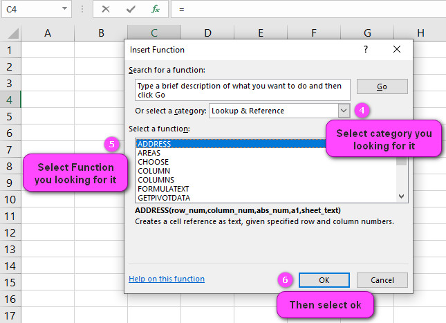
We can find this function in Lookup & reference of insert function Tab.

How to use SORTBY function in excel

1. Click on empty cell (like F5).

2. Click on fx icon (or press shift+F3).

3. In insert function tab you will see all functions.

4. Select Lookup & reference category.

5. Select SORTBY function.

6. Then select ok.

7. In function arguments Tab, you will see SORTBY function.

8. Lookup value is a value that SORTBY searches for in Lookup vector and can be a number,text, a logical value, or a name or reference to a value.

9. Lookup vector is a range that contains only one row or one column of text, numbers, or logical values, placed in ascending order.

10. Result vector is a range that contains only one row or column, the same size as lookup vector.

11. Lookup value is a value that LOOKUP searches for in Array and can be a number, text, a logical value, or a name or reference to a value.

12. Array is a range of cells that contain text, number, or logical values that you want to compare with Lookup value.

13. You will see the result in formula result section.

Examples of SORTBY function in excel

Here are a few examples of using the SORTBY function in Microsoft Excel:

Example 1: Sorting by a single column Suppose you have a table with four columns: Region, Salesperson, Product, and Sales Amount.

To sort the table by Sales Amount in descending order, you would use the following formula:

=SORTBY(A2:D10, D2:D10, -1)

In this formula, A2:D10 is the range of cells that you want to sort. The second argument, D2:D10, specifies the column to sort by – Sales Amount (column D).

The third argument, -1, indicates that the data should be sorted in descending order.

Example 2: Sorting by multiple columns Suppose you have a table with three columns: Name, Age, and Score.

To sort the table first by age in ascending order, and then within each age group, by score in descending order, you would use the following formula:

=SORTBY(A2:C11, {B2:B11, -C2:C11}, {TRUE, FALSE})

In this formula, A2:C11 is the range of cells that you want to sort. The second argument, {B2:B11, -C2:C11}, specifies the two columns to sort by – Age (column B) and Score (column C).

The “-” operator before the Score column reference indicates that it should be sorted in descending order.

The third argument, {TRUE, FALSE}, specifies the sorting order for each column – TRUE for ascending order (for the Age column) and FALSE for descending order (for the Score column).

Example 3: Sorting by date or time values Suppose you have a table with four columns: Region, Salesperson, Product, and Sale Date.

To sort the table by Sale Date in ascending order, you would use the following formula:

=SORTBY(A2:D10, D2:D10)

In this formula, A2:D10 is the range of cells that you want to sort. The second argument, D2:D10, specifies the column to sort by – Sale Date (column D).

Since the Sale Date column contains date values, Excel will automatically recognize these as dates and sort them chronologically.

Example 4: Sorting with a filter applied Suppose you have a table with three columns: Name, Age, and Score.

To sort the table by Score in descending order, but exclude any rows where the Age is less than 18, you would use the following formula:

=SORTBY(FILTER(A2:C11, B2:B11>=18), FILTER(C2:C11, B2:B11>=18), -1)

In this formula, FILTER is used to create a new range that only includes the rows where the Age is greater than or equal to 18.

This filtered data is then sorted by the Score column in descending order, using the SORTBY function.

How do I use the SORTBY function in Excel?

The SORTBY function in Microsoft Excel allows you to sort a range of data based on one or more columns that you specify.

Here is a step-by-step guide on how to use the SORTBY function in Excel:

1. Start by selecting the range of cells that you want to sort.
2. In the formula bar, type “=SORTBY(” and then select the range of cells that you want to sort.
3. Next, add a comma after the first argument, and then specify the column or columns that you want to sort by.
   • You can enter a single column reference or multiple column references separated by commas.
4. If you want to sort in ascending order, add another comma after the column reference(s) and enter “TRUE”.
   • If you want to sort in descending order, enter “FALSE” instead.
5. Close the formula with a closing parenthesis “)” and press Enter.

Here is an example of how to use the SORTBY function:

Suppose you have a table of sales data for different regions and you want to sort it based on the sales amount in descending order.

The table has four columns: Region, Salesperson, Product, and Sales Amount.

To sort the data, you would follow these steps:

1. Select the entire table, including headings.
2. Type “=SORTBY(” in an empty cell outside the table and select the entire table.
3. Enter a comma, and then specify the column containing the sales amount (column D).
4. Enter “FALSE” to sort in descending order.
5. Close the formula with “)” and press Enter.

The sorted table will now be displayed in descending order based on the sales amount column.

What are the arguments of the SORTBY function?

The SORTBY function in Microsoft Excel has two arguments:

1. range: This is the range of cells you want to sort. It can be a single column or multiple columns.
2. [sort_by]: This is the reference to one or more columns that you want to sort the data by.
   • You can specify one or multiple columns separated by commas.

The sort_by argument is an optional argument. If it is not specified, Excel will sort the range based on the first column by default.

The sort_by argument can also take an array of values as input. In this case, the function will sort the data based on multiple columns at once.

For example, if you want to sort a table of sales data by region and then by sales amount within each region, you can use the following formula:

= SORTBY(A2:D10, {A2:A10, D2:D10}, {TRUE, FALSE})

In this example, the sort_by argument is an array containing two columns – the region column (A2:A10) and the sales amount column (D2:D10).

The curly braces around the array indicate that it is an array constant. The second argument of the SORTBY function specifies the sorting order for each column – TRUE for ascending and FALSE for descending.

This formula would sort the data first by region in ascending order, and then within each region, by sales amount in descending order.

In summary, the SORTBY function takes a range of data as the first argument and one or more columns to sort by as the second argument.

The sort_by argument can be a single column or an array of multiple columns, and it can also specify the sorting order for each column.

Can I sort by multiple columns using the SORTBY function?

Yes, you can sort by multiple columns using the SORTBY function in Microsoft Excel.

To do this, you simply need to specify the reference to multiple columns in the second argument of the SORTBY function.

Here is an example of how to sort a table of sales data by two columns using the SORTBY function:

Suppose you have a table with four columns: Region, Salesperson, Product, and Sales Amount.

You want to sort the table first by Region in ascending order, and then within each region, by Sales Amount in descending order.

To do this, you would use the following formula:

= SORTBY(A2:D10, {A2:A10, D2:D10}, {TRUE, FALSE})

In this formula, A2:D10 is the range of cells that you want to sort. The second argument, {A2:A10, D2:D10}, specifies the two columns to sort by – Region (column A) and Sales Amount (column D).

The curly braces around the array indicate that it is an array constant. The third argument, {TRUE, FALSE}, specifies the sorting order for each column – TRUE for ascending order (for the Region column) and FALSE for descending order (for the Sales Amount column).

When you press Enter, the SORTBY function will sort the table first by the Region column in ascending order, and then within each region, by the Sales Amount column in descending order.

In summary, you can use the SORTBY function to sort a range of cells by multiple columns.

Simply provide a reference to each column you want to sort by in an array as the second argument of the function.

How do I sort data in descending order using the SORTBY function?

To sort data in descending order using the SORTBY function in Microsoft Excel, you need to add the “FALSE” argument to the second argument of the function.

This indicates that the data should be sorted in descending order.

Here is an example of how to use the SORTBY function to sort a table of sales data by Sales Amount in descending order:

Suppose you have a table with four columns: Region, Salesperson, Product, and Sales Amount.

To sort the table by Sales Amount in descending order, you would use the following formula:

= SORTBY(A2:D10, D2:D10, FALSE)

In this formula, A2:D10 is the range of cells that you want to sort.

The second argument, D2:D10, specifies the column to sort by – Sales Amount (column D).

The third argument, FALSE, indicates that the data should be sorted in descending order.

When you press Enter, the SORTBY function will sort the table by Sales Amount in descending order.

Alternatively, you can also use the “-” operator before the column reference to sort the data in descending order.

For example, you can rewrite the above formula as follows:

= SORTBY(A2:D10, -D2:D10)

This formula achieves the same result as the previous one – sorting the table by Sales Amount in descending order.

In summary, to sort data in descending order using the SORTBY function, you need to specify the column reference in the second argument of the function and add a “FALSE” argument or use the “-” operator before the column reference to indicate that the data should be sorted in descending order.

Can I use the SORTBY function to sort by date or time values?

Yes, you can use the SORTBY function in Microsoft Excel to sort by date or time values.

The SORTBY function can sort a range of cells based on any data type, including dates and times.

Here is an example of how to use the SORTBY function to sort a table of sales data by date:

Suppose you have a table with four columns: Region, Salesperson, Product, and Sale Date.

To sort the table by Sale Date, you would use the following formula:

= SORTBY(A2:D10, D2:D10)

In this formula, A2:D10 is the range of cells that you want to sort. The second argument, D2:D10, specifies the column to sort by – Sale Date (column D).

Since the Sale Date column contains date values, Excel will automatically recognize these as dates and sort them chronologically.

If you want to sort the data in reverse chronological order, you can add the “FALSE” argument to the SORTBY function, like this:

= SORTBY(A2:D10, D2:D10, FALSE)

This will sort the data in descending order based on the Sale Date column.

Similarly, if you have a column containing time values, you can sort the data using the SORTBY function in the same way.

For example, suppose you have a table with four columns: Region, Salesperson, Product, and Time Taken. To sort the table by Time Taken, you would use the following formula:

= SORTBY(A2:D10, D2:D10)

In this formula, A2:D10 is the range of cells that you want to sort.

The second argument, D2:D10, specifies the column to sort by – Time Taken (column D).

Since the Time Taken column contains time values, Excel will automatically recognize these as times and sort them chronologically.

In summary, you can use the SORTBY function to sort a range of cells based on any data type, including dates and times.

Simply specify the column containing the date or time values in the second argument of the function, and Excel will automatically recognize these as dates or times and sort them accordingly.

What happens if the range provided to the SORTBY function contains blank cells?

If the range provided to the SORTBY function contains blank cells, the SORTBY function will treat those cells as if they contain a value of zero (0) or an empty string (“”).

This means that any blank cells in the range will be treated as if they are at the beginning or end of the sorted range, depending on whether the sorting order is ascending or descending.

Here is an example of how the SORTBY function handles blank cells:

Suppose you have a table with two columns: Name and Score.

The Score column contains some blank cells. To sort the table by Score in ascending order, you would use the following formula:

= SORTBY(A2:B11, B2:B11)

In this formula, A2:B11 is the range of cells that you want to sort. The second argument, B2:B11, specifies the Score column as the column to sort by.

If there are blank cells in the Score column, Excel will treat them as if they contain a value of zero (0).

Therefore, any rows with a blank score will appear at the beginning of the sorted range if the sorting order is ascending.

Alternatively, if you want to sort the data in descending order, you can use the following formula:

= SORTBY(A2:B11, B2:B11, FALSE)

In this case, any rows with a blank score will appear at the end of the sorted range.

It’s worth noting that if you want to exclude blank cells from the sorted range entirely, you can do so by using the FILTER function to create a new range that only includes non-blank cells.

For example, if you want to sort the Score column but exclude any blank cells, you can use the following formula:

= SORTBY(FILTER(B2:B11, B2:B11<>””), FILTER(A2:B11, B2:B11<>””))

This formula uses the FILTER function to create a new range that only includes non-blank cells in the Score column, and then sorts the filtered range while preserving the corresponding values in the Name column.

In summary, if the range provided to the SORTBY function contains blank cells, those cells will be treated as if they contain a value of zero (0) or an empty string (“”).

The position of the blank cells in the sorted range will depend on the sorting order specified in the formula.

Can the SORTBY function be used with other functions in Excel?

Yes, the SORTBY function in Microsoft Excel can be used with other functions to perform more complex calculations and data analysis.

Here are some examples of how you can use the SORTBY function with other functions:

1. AVERAGEIFS: You can use the AVERAGEIFS function to calculate the average value of a column based on multiple criteria, and then sort the results using SORTBY.
   • For example, suppose you have a table with four columns: Region, Salesperson, Product, and Sales Amount.
   • To calculate the average sales amount for each region and sort the results in descending order, you would use the following formula:

= SORTBY(AVERAGEIFS(D2:D10, A2:A10, {“East”, “West”}), {“East”, “West”}, FALSE)

This formula first uses the AVERAGEIFS function to calculate the average sales amount for each region (East and West).

The results are then sorted using SORTBY in descending order based on the corresponding regions.

2. INDEX & MATCH: You can use the INDEX and MATCH functions together with SORTBY to retrieve specific values from a sorted range.
   • For example, suppose you have a table with three columns: Name, Age, and Score. To retrieve the name of the person with the highest score, you would use the following formula:

= INDEX(A2:A11, MATCH(MAX(B2:B11), SORTBY(B2:B11, B2:B11, FALSE), 0))

This formula first uses SORTBY to sort the Score column in descending order.

The MAX function is then used to find the highest score in the sorted range.

Finally, the INDEX and MATCH functions are used together to retrieve the name of the person with the highest score.

3. COUNTIFS: You can use the COUNTIFS function to count the number of cells that meet multiple criteria, and then sort the results using SORTBY.
   • For example, suppose you have a table with two columns: Name and Score.
   • To count the number of people who scored above 80, you would use the following formula:

= SORTBY(COUNTIFS(B2:B11, “>80”, A2:A11, “<>”), COUNTIFS(B2:B11, “>80”, A2:A11, “<>”), FALSE)

This formula first uses the COUNTIFS function to count the number of cells in the Score column that are greater than 80 and have a corresponding non-blank cell in the Name column.

The results are then sorted using SORTBY in descending order based on the corresponding counts.

In summary, the SORTBY function can be used with other functions in Microsoft Excel to perform more complex calculations and data analysis.

Some common functions that can be used with SORTBY include AVERAGEIFS, INDEX & MATCH, and COUNTIFS.

How does the SORTBY function differ from the traditional SORT function in Excel?

The SORTBY function in Microsoft Excel is an evolution of the traditional SORT function, with some key differences in terms of functionality and usage.

Here are some of the main differences between the SORTBY and SORT functions:

1. Range selection: The SORTBY function allows you to sort a range of cells based on a specific column or multiple columns.
   • In contrast, the SORT function only allows you to sort a single row or column of data.
2. Sorting order: The SORTBY function allows you to specify the sorting order for each column individually.
   • In contrast, the SORT function only allows you to sort data in either ascending or descending order.
3. Preserving data integrity: The SORTBY function maintains the relationship between rows when sorting by multiple columns, ensuring that data integrity is preserved.
   • In contrast, the SORT function does not preserve relationships between rows, which can lead to data inconsistencies.
4. Efficiency: The SORTBY function is generally more efficient than the SORT function when sorting large datasets.
   • This is because the SORTBY function only needs to access the data once, whereas the SORT function may need to access the data multiple times to perform the sorting operation.

Here is an example of how the SORTBY function differs from the traditional SORT function:

Suppose you have a table with three columns: Name, Age, and Score.

To sort the table first by age in ascending order, and then within each age group, by score in descending order, you would use the following formula with the SORTBY function:

= SORTBY(A2:C11, {B2:B11, -C2:C11}, {TRUE, FALSE})

In this formula, A2:C11 is the range of cells that you want to sort. The second argument, {B2:B11, -C2:C11}, specifies the two columns to sort by – Age (column B) and Score (column C).

The “-” operator before the Score column reference indicates that it should be sorted in descending order.

The third argument, {TRUE, FALSE}, specifies the sorting order for each column – TRUE for ascending order (for the Age column) and FALSE for descending order (for the Score column).

In contrast, to sort the same table using the traditional SORT function, you would use the following formula:

= SORT(B2:C11, 2, TRUE, 3, FALSE)

This formula sorts the data by the second column (Age) in ascending order, and then by the third column (Score) in descending order.

However, the SORT function does not preserve relationships between rows, which means that any details of Age will not remain the same.

In summary, the SORTBY function in Excel is a more advanced and efficient sorting function than the traditional SORT function.

It allows for sorting by multiple columns, preserving relationships between rows, and specifying sorting orders for each column individually, making it a more flexible tool for data analysis.

Are there any limitations or known issues with using the SORTBY function in Excel?

While the SORTBY function in Microsoft Excel is a powerful tool for sorting data, there are some limitations and known issues that you should be aware of when using it.

Here are some of the main limitations and issues with using the SORTBY function:

1. Only available in newer versions of Excel: The SORTBY function is only available in newer versions of Excel, such as Excel 365, Excel 2019, and Excel 2016 (with certain updates).
   • If you’re using an older version of Excel, you won’t be able to use the SORTBY function.
2. Requires a single contiguous range: The SORTBY function requires that the range you want to sort is a single contiguous range.
   • This means that if you want to sort data from multiple non-adjacent ranges, you’ll need to use the CONCAT or UNION functions to combine them into a single range first.
3. Limited to 64,000 rows: The SORTBY function has a limit of 64,000 rows for each column that you’re sorting by.
   • If your data exceeds this limit, you’ll need to split it into smaller chunks and sort each chunk separately.
4. May cause calculation delays: Sorting large datasets using the SORTBY function can cause calculation delays, particularly if you’re using other functions or formulas that reference the sorted data.
   • To minimize these delays, you may need to adjust your settings or use more efficient formulas.
5. May not work as expected with certain data types: In rare cases, the SORTBY function may not work as expected with certain data types, such as text strings or mixed data types.
   • If you encounter unexpected results, try converting the data to a different format before sorting.

In summary, while the SORTBY function in Excel is a powerful tool for sorting data, there are some limitations and known issues that you should be aware of when using it.

By understanding these limitations and working around them when necessary, you can make the most of this function and use it effectively in your data analysis.

Related posts:

Discounted cash flow excel Excel COLUMN Function How to Use Chat GPT with Excel Creating Infographics with Excel