What is SUMSQ Function in Excel?
The SUMSQ function is one of the math functions of Excel.
It Returns the sum of the squares of the arguments.
The arguments can be numbers, arrays, names, or references to cells that contain numbers.
We can find this function in Math & trig category of insert function Tab.
How to use SUMSQ function in excel
- Click on an empty cell (like F5 )

2. Click on fx icon (or press shift+F3)

3. In the insert function tab you will see all functions

4. Select math and trig category
5. Select SUMSQ function
6. Then select ok

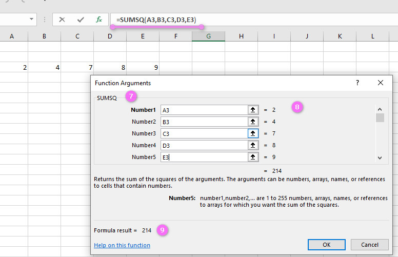
7. In the function arguments Tab you will see SUMSQ function
8. Number1,number2,… are 1 to 255 numbers, arrays, names, or references to arrays for which you want the sum of the squares.
This function first obtains the square of each of the input values and then adds them together.
9. You will see results in the formula result section
Examples of SUMSQ function in Excel
- To find the sum of squares of a range of numbers, enter the following formula:
=SUMSQ(A2:A10) - To find the sum of squares for multiple ranges of numbers, enter the following formula:
=SUMSQ(A2:A10,B2:B10,C2:C10) - To find the sum of squares for a dynamic range of numbers, enter the following formula:
=SUMSQ(INDIRECT("A2:A"&COUNT(A:A)+1)) - To find the sum of squares for a filtered range of numbers, enter the following formula:
=SUMSQ(SUBTOTAL(9,A2:A100)*A2:A100) - To find the sum of squares for non-numeric values in a range, use the IFERROR function to exclude them from the calculation:
=SUMSQ(IFERROR(A2:A10^2,0)) - To find the sum of squares for a range of negative numbers, use the ABS function to convert them to positive numbers before squaring them:
=SUMSQ(ABS(A2:A10))^2 - To find the sum of squares for a range of decimals, use the ROUND function to round them to a specified number of decimal places before squaring them:
=SUMSQ(ROUND(A2:A10,2))^2 - To find the sum of squares for a range of time durations, use the HOUR, MINUTE, and SECOND functions to convert them to seconds before squaring them:
=SUMSQ((HOUR(A2:A10)*3600+MINUTE(A2:A10)*60+SECOND(A2:A10))^2) - To find the sum of squares for a range of cell references that contain formulas, use the VALUE function to convert them to values before squaring them:
=SUMSQ(VALUE(A2:A10))^2 - To find the sum of squares for a range of numbers using an array formula, enter the following formula and press Ctrl + Shift + Enter:
{=SUMSQ(A2:A10)}
Example 1:
How to use SUMSQ function in excel
You can see examples of SUMSQ function below:
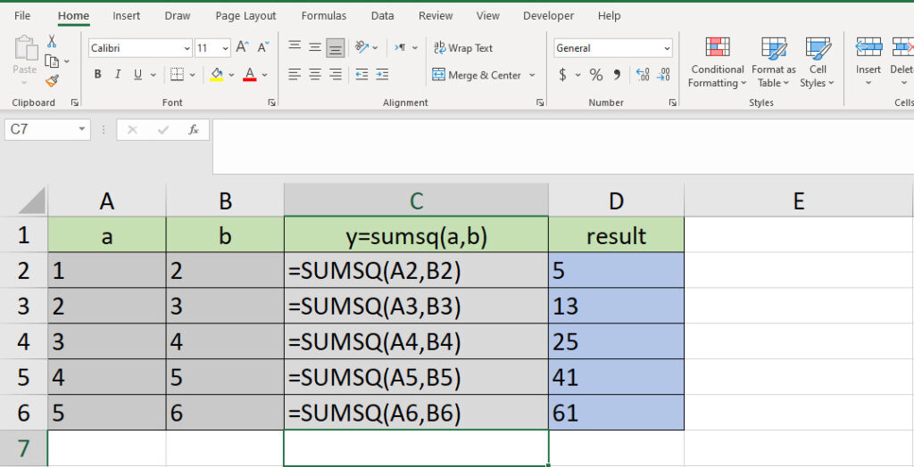
sumsq(A2,B2) ----->>>>answer is  5

sumsq(A3,B3) ----->>>>answer is  13

sumsq(A4,B4) ----->>>>answer is  25

sumsq(A5,B5) ----->>>>answer is  41

sumsq(A6,B6) ----->>>>answer is  61
“Excel’s SUMSQ Function: A Powerful Tool for Calculating Sum of Squares”
The SUMSQ function in Excel is a powerful tool for calculating the sum of squares for a given set of numbers. It takes in one or more arguments, which can be numeric values, cell references, or ranges, and returns the sum of squares of those values.
For example, suppose you have a data set containing the following numbers:
1, 2, 3, 4, 5
To calculate the sum of squares for this data set, you can use the SUMSQ function as follows:
=SUMSQ(1,2,3,4,5)
This will return the result: 55, which represents the sum of squares of all the numbers in the data set.
“Understanding the Inner Workings of Excel’s SUMSQ Function”
The SUMSQ function works by first squaring each number in the input range, and then summing up the squares of all the numbers to compute the final result. It essentially calculates the variance of the input values.
For example, consider the same data set as above. The squared values of these numbers would be:
1^2 = 1 2^2 = 4 3^2 = 9 4^2 = 16 5^2 = 25
Adding these squared values gives us a total of 55, which is the same result returned by the SUMSQ function.
“Mastering the Arguments of the SUMSQ Function in Excel”
The SUMSQ function can take one or more arguments, which can be individual values, cell references, or ranges. You can combine these arguments in any way you like to compute the sum of squares of multiple sets of data.
For example, suppose you have two data sets: one containing the numbers (1, 2, 3) and another containing the numbers (4, 5, 6). You can calculate the sum of squares for both data sets using the following formula:
=SUMSQ(1,2,3)+SUMSQ(4,5,6)
This will return the result: 91, which represents the sum of squares of all the numbers in both data sets.
“When to Use the SUMSQ Function in Excel for Data Analysis”
The SUMSQ function is useful when you need to compute the variance of a set of data. Variance is a measure of how spread out a set of data is from its average value. The larger the variance, the more spread out the data is.
For example, suppose you have a set of test scores for a group of students. You can use the SUMSQ function to compute the variance of these scores, which can help you understand how much variation there is in the scores.
To calculate the variance of the test scores using the SUMSQ function, you first need to calculate the mean (average) of the scores using the AVERAGE function. Then, you can use the following formula:
=SUMSQ(A1:A10)/(COUNT(A1:A10)-1)
Here, A1:A10 is the range containing the test scores, and COUNT(A1:A10)-1 is the degrees of freedom for the sample. This formula will give you the variance of the test scores.
“Summing up Negative Numbers and Decimals with Excel’s SUMSQ Function”
The SUMSQ function works with both positive and negative numbers, as well as decimal numbers. When working with negative numbers, the squared values of those numbers are positive, so they contribute to the final result just like positive numbers.
For example, suppose you have a data set containing the following numbers:
-1, 2, -3, 4, -5
To calculate the sum of squares for this data set, you can use the SUMSQ function as follows:
=SUMSQ(-1,2,-3,4,-5)
This will return the result: 55, which represents the sum of squares of all the numbers in the data set, including negative numbers.
“Combining Functions with Excel’s SUMSQ for Advanced Data Analysis”
The SUMSQ function in Excel can be combined with other functions to perform advanced data analysis. For example, you can use it with the AVERAGE function to compute the standard deviation of a set of data.
To calculate the standard deviation of a set of test scores using the SUMSQ and AVERAGE functions, you can use the following formula:
=SQRT(SUMSQ(A1:A10)/(COUNT(A1:A10)-1))
Here, A1:A10 is the range containing the test scores, and COUNT(A1:A10)-1 is the degrees of freedom for the sample. This formula will give you the standard deviation of the test scores.
“The Case Sensitivity of Excel’s SUMSQ Function: What You Need to Know”
The SUMSQ function in Excel is not case-sensitive. This means that it treats uppercase and lowercase letters as equivalent when evaluating criteria.
For example, suppose you have a data set containing the following strings:
“apple”, “Apple”, “APPLE”
To count the number of occurrences of the word “apple” in this data set using the SUMSQ function, you can use the following formula:
=SUMSQ(COUNTIF(A1:A10,”apple”),COUNTIF(A1:A10,”Apple”),COUNTIF(A1:A10,”APPLE”))
This will return the result: 3, which represents the total number of occurrences of the word “apple” in the data set, regardless of case.
“How to Handle Errors and Blank Cells While Using Excel’s SUMSQ Function”
When using the SUMSQ function in Excel, blank cells and errors such as #REF!, #VALUE! or #NAME! can affect the accuracy of the result. To handle these issues, you can use the IFERROR function to replace error values with a specified value, and the ISBLANK function to exclude blank cells from the calculation.
For example, suppose you have a data set containing some blank cells and errors. To calculate the sum of squares for this data set while handling these issues, you can use the following formula:
=SUMSQ(IFERROR(A1:A10^2,0))
This formula replaces any error values with 0 and sums up the squares of all non-blank cells in the range A1:A10.
“The Importance of Argument Order in Excel’s SUMSQ Function”
The order of arguments in the SUMSQ function in Excel is important, as it affects the accuracy of the result. The first argument should be the range of cells to be squared; subsequent arguments should be blank or omitted.
For example, suppose you have a data set containing the following numbers:
3, 5, 7
To calculate the sum of squares for this data set using the SUMSQ function, you can use the following formula:
=SUMSQ(A1:A3)
This formula adds up the squares of all the numbers in the range A1:A3.
“Calculating Variance with Excel’s SUMSQ Function: A Step-by-Step Guide”
The SUMSQ function in Excel can be used to calculate variance by dividing the sum of squares by the degrees of freedom for the sample. The degrees of freedom are equal to the number of data points minus one.
For example, suppose you have a set of test scores for a group of students. To calculate the variance of these scores using the SUMSQ function, you can follow these steps:
- Calculate the mean (average) of the scores using the AVERAGE function.
- Subtract the mean from each score to get the deviations from the mean.
- Square each deviation to get the squares of the deviations.
- Add up the squares of the deviations using the SUMSQ function.
- Divide the sum of squares by the degrees of freedom for the sample (i.e. the number of data points minus one) to get the variance.
The formula for calculating variance using the SUMSQ function is:
=SUMSQ(A1:A10)/(COUNT(A1:A10)-1)
Here, A1:A10 is the range containing the test scores, and COUNT(A1:A10)-1 is the degrees of freedom for the sample. This formula will give you the variance of the test scores.
“Using Excel’s SUMSQ Function for Standard Deviation Calculation”
Excel’s SUMSQ function can be used to calculate the sum of squares, which is a crucial component in the calculation of standard deviation. To calculate the standard deviation of a set of data using the SUMSQ function in Excel, you need to divide the sum of squares by the sample size minus one, and then take the square root of the result.
For example, suppose you have a set of test scores for a group of students in cells A1:A10. To calculate the standard deviation of these scores using the SUMSQ function, you can use the following formula:
=SQRT(SUMSQ(A1:A10)/(COUNT(A1:A10)-1))
This formula will give you the standard deviation of the test scores.
“Comparing Two Sets of Data with Excel’s SUMSQ Function”
You can use the SUMSQ function in Excel to compare two sets of data by calculating the sum of squares for both sets separately, and then comparing the results. The set with the higher sum of squares will have a larger variance and more spread out data.
For example, suppose you have two sets of test scores for two different classes of students: Class A and Class B. You want to know which class has more spread out test scores. You can calculate the sum of squares for both sets of test scores using the SUMSQ function as follows:
=SUMSQ(A1:A10) =SUMSQ(B1:B10)
This will give you the sum of squares for both sets of test scores. You can then compare the results to see which set has a higher sum of squares, indicating more spread out data.
“Nesting the SUMSQ Function within Other Functions in Excel”
The SUMSQ function in Excel can be nested within other functions to perform more advanced calculations. For example, you can use the SUMSQ function with the IF function to calculate the sum of squares for a specific set of data based on certain criteria.
For example, suppose you have a data set in cells A1:A10, and you want to calculate the sum of squares for all the numbers greater than 5. You can use the following formula:
=SUMSQ(IF(A1:A10>5,A1:A10,0))
This formula evaluates each value in the range A1:A10 against the criterion (greater than 5) and returns the sum of squares for all values that meet the criterion.
“Extracting Root Mean Square with Excel’s SUMSQ Function”
The SUMSQ function in Excel can be used to extract the root mean square (RMS) of a set of data. The RMS is the square root of the average of the sum of squares of a set of values.
For example, suppose you have a data set containing the following numbers:
1, 2, 3, 4, 5
To calculate the RMS of this data set using the SUMSQ function, you can use the following formula:
=SQRT(SUMSQ(A1:A5)/COUNT(A1:A5))
Here, A1:A5 is the range containing the data set, and COUNT(A1:A5) is the number of data points in the set. This formula will give you the RMS of the data set.
“Dynamic Range Calculations with Excel’s SUMSQ Function”
Excel’s SUMSQ function can be used for dynamic range calculations by combining it with other functions such as OFFSET or INDEX. This allows you to calculate the sum of squares for a range of data that changes in size or location over time.
For example, suppose you have a data set in cells A1:A10, but the size of the data set changes every week. You can use the OFFSET function to create a dynamic range that adjusts to the size of the data set, and then use the SUMSQ function to calculate the sum of squares for this range. The formula would be:
=SUMSQ(OFFSET(A1,0,0,COUNTA(A:A),1))
“Calculating Correlation Coefficient with Excel’s SUMSQ Function”
Excel’s SUMSQ function can be used to calculate the correlation coefficient between two sets of data. The correlation coefficient measures the strength and direction of the linear relationship between two variables.
For example, suppose you have two sets of data in cells A1:A10 and B1:B10. To calculate the correlation coefficient between these two sets of data using the SUMSQ function in Excel, you can use the following formula:
=SUMPRODUCT(A1:A10,B1:B10)/SQRT(SUMSQ(A1:A10)*SUMSQ(B1:B10))
This formula calculates the sum of product of the two sets of data and divides it by the square root of the product of the sum of squares of each of the two sets of data.
“Analyzing Large Datasets with Excel’s SUMSQ Function”
Excel’s SUMSQ function is a powerful tool for analyzing large datasets. It can quickly compute the sum of squares for a large number of data points, allowing you to identify patterns and trends that would be difficult to see otherwise.
For example, suppose you have a dataset containing the daily sales figures for a retail store for the past year. This dataset contains thousands of data points, making it difficult to analyze. By using the SUMSQ function in Excel, you can quickly calculate the sum of squares of this dataset, which can help you identify trends and patterns in the sales figures.
“Statistical Analysis Made Easy with Excel’s SUMSQ Function”
Excel’s SUMSQ function makes statistical analysis easy by providing a simple way to calculate sums of squares. Sums of squares are a key component in many statistical calculations, including calculating variance, standard deviation, and correlation coefficients.
For example, suppose you have a set of test scores for a group of students. You can use the SUMSQ function to calculate the variance of these scores, which can help you understand how much variation there is in the scores. You can then use this information to make informed decisions about how to improve the students’ performance.
“Regression Analysis with Excel’s SUMSQ Function: A Comprehensive Overview”
Excel’s SUMSQ function is a key component in regression analysis, which is a statistical technique used to identify relationships between variables. In regression analysis, the SUMSQ function is used to calculate the sum of squares of the residuals, which are the differences between the observed values and the predicted values.
For example, suppose you have a dataset containing the heights and weights of a group of people. You can use the SUMSQ function to perform a regression analysis to determine if there is a relationship between height and weight. The SUMSQ function would be used to calculate the sum of squares of the residuals, which would indicate how well the regression line fits the data.
“Exploring the Limitations of Excel’s SUMSQ Function”
While Excel’s SUMSQ function is a powerful tool for statistical analysis, it has some limitations. One limitation is that it only works with numeric values, so non-numeric values such as text or logical values will cause errors. Another limitation is that it cannot handle missing data points, which can affect the accuracy of the result.
For example, suppose you have a set of data containing some missing values. If you try to calculate the sum of squares using the SUMSQ function, you may get inaccurate results due to the missing data points. To handle missing data points, you can use functions such as AVERAGEIF or IFERROR to replace missing values with a specified value before calculating the sum of squares.
