What is VLOOKUP function in Excel?
The VLOOKUP function is one of the Lookup & reference functions of Excel.
It looks for a value in the leftmost column of a table and then returns a value in the same row from a column you specify.
By default, the table must be sorted in ascending order.
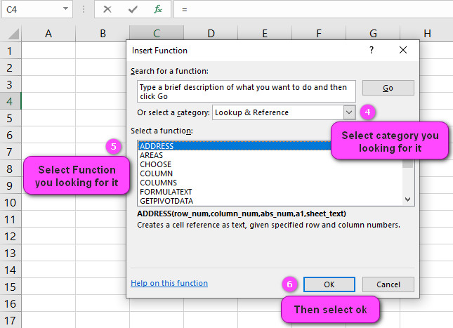
We can find this function in Lookup & reference category of insert function Tab.
How to use VLOOKUP function in excel
- Click on an empty cell (like F5).

2. Click on the fx icon (or press shift+F3).

3. In the insert function tab you will see all functions.

4. Select Lookup & reference category.
5. Select VLOOKUP function
6. Then select ok.
7. In function arguments Tab, you will see VLOOKUP function.
8. Lookup value is the value to be found in the first column of the table, and can be a value, a reference, or a text string.
9. Table_array is a table of text, numbers, or logical values, in which data is retrieved. Table_array can be a reference to a range or a range name.
10. Col_index_num is the column number in table array from which the matching value should be returned. The first column of values in the table is column 1.
11. Range lookup is a logical value: to find the closest match in the first column (sorted in ascending order) = TRUE or omitted; find an exact match = FALSE.

12. You will see the result in the formula result section.
Examples of VLOOKUP function in excel
Example 1:
Find the unique characteristics of a person in the table
We want to find the height, age, and weight of a person named “Elijah” from the following data

VLOOKUP(H4,A2:E10,2,FALSE)----->>>>answer is  22
VLOOKUP(H4,A2:E10,3,FALSE)----->>>>answer is  198
VLOOKUP(H4,A2:E10,4,FALSE)----->>>>answer is  185
VLOOKUP(H4,A2:E10,5,FALSE)----->>>>answer is  175
Example 2:
Is vlookup vertical or horizontal in excel?
The vlookup function searches the data vertically in the table. We use the Hlookup function to search the data horizontally.

=VLOOKUP(H4,A2:E10,2,FALSE)----->>>>answer is  22
=VLOOKUP(H4,A2:E10,3,FALSE)----->>>>answer is  198
=VLOOKUP(H4,A2:E10,4,FALSE)----->>>>answer is  185
=VLOOKUP(H4,A2:E10,5,FALSE)----->>>>answer is  175
Example 3:
VLOOKUP is based on column or row numbers?
This function finds the desired data in the table based on the number of columns.

This function counts the number of cells from the left side and when it reaches the desired number, it displays the result in the output.
=VLOOKUP(H4,A2:E10,2,FALSE)----->>>>answer is  22
=VLOOKUP(H4,A2:E10,3,FALSE)----->>>>answer is  198
=VLOOKUP(H4,A2:E10,4,FALSE)----->>>>answer is  185
=VLOOKUP(H4,A2:E10,5,FALSE)----->>>>answer is  175
Example 4:
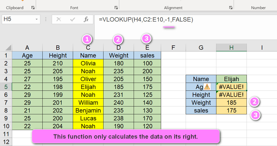
Does the VLOOKUP function search the values on the right or the values on the left?
This function only calculates the data on its right.

=VLOOKUP(H4,A2:E10,-1,FALSE)----->>>>answer is #VALUEExample 5:
What is the difference between an exact match and an approximate match in VLOOKUP?
Example 6:
Does the VLOOKUP function find all the desired items in the table or only the first value?
This function only finds the first case that meets the desired condition. In the example below, there are three nouns called “Noah”, and the Vlookup function only searches for the first one.

=VLOOKUP(H4,A2:E10,2,FALSE)----->>>>answer is  25
=VLOOKUP(H4,A2:E10,3,FALSE)----->>>>answer is  205
=VLOOKUP(H4,A2:E10,4,FALSE)----->>>>answer is  235
=VLOOKUP(H4,A2:E10,5,FALSE)----->>>>answer is  200
Example 7:
Combination of two functions VLOOKUP and IFNA
If the output of the Vlookup function gives an error, the IFNA function can be used.

=IFNA(VLOOKUP(H4,A2:E10,2,FALSE),"not exist")--->>>>answer is not existWhat is the purpose of VLOOKUP function?
It looks for a value in the leftmost column of a table and then returns a value in the same row from a column you specify
What is the Return value of VLOOKUP function?
It can return any type of data.
VLOOKUP(Lookup value,Table_array,Col_index_num,Rangelookup)=number,textHow many arguments does VLOOKUP function have?
VLOOKUP(Lookup value,Table_array,Col_index_num,Rangelookup)=number,textThis function has just 4 Arguments.
Lookup value is the value to be found in the first column of the table
Table_array is a table of text, numbers, or logical values, in which data is retrieved.
Col_index_num is the column number in the table array from which the matching value should
be returned.
Range lookup is a logical value: to find the closest match in the first column (sorted in
ascending order) = TRUE or omitted; find an exact match = FALSE
Range lookup argument of VLOOKUP function is optional.
Which version of Excel supports VLOOKUP function?
This function is available for all excel versions (2003-2019)
Errors in VLOOKUP function
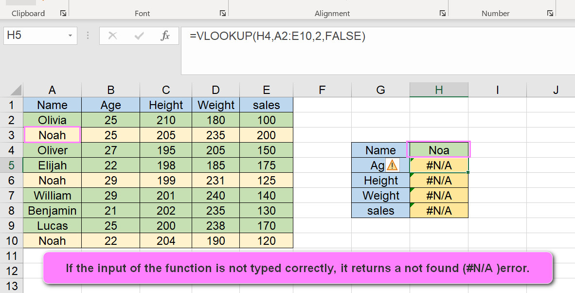
If the VLOOKUP function does not find any items, it returns a not found (#N/A ) error.

VLOOKUP(H4,A2:E10,2,FALSE)----->>>>answer is #N/AIf the input of the function is not typed correctly, it returns a not found (#N/A ) error.
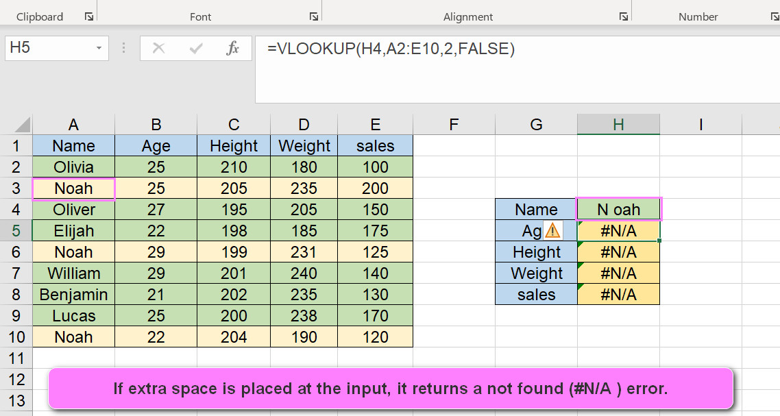
VLOOKUP(H4,A2:E10,2,FALSE)----->>>>answer is #N/AIf extra space is placed at the input, it returns a not found (#N/A ) error.
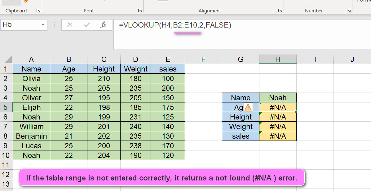
VLOOKUP(H4,A2:E10,2,FALSE)----->>>>answer is #N/AIf the table range is not entered correctly, it returns a not found (#N/A ) error.
VLOOKUP(H4,A2:E10,2,FALSE)----->>>>answer is #N/AIf the Col_index_num is not entered correctly, it returns a not found (#VALUE) error.
=VLOOKUP(H4,A2:E10,-1,FALSE)----->>>>answer is #VALUEHow do I use the VLOOKUP function in Excel?
Sure, here’s a complete explanation with examples on how to use the VLOOKUP function in Excel.
The VLOOKUP function is used to search for a specific value in the first column of a range or table, and then return a corresponding value from another column in the same row.
This function is commonly used to look up information in a large dataset or table.
The syntax of the VLOOKUP function is as follows:
=VLOOKUP(lookup_value,table_array,col_index_num,[range_lookup])
lookup_valueis the value that you want to find in the first column of the table.table_arrayis the range or table where you want to search for the lookup value.col_index_numis the number of the column in the table where you want to return the result.- For example, if you want to return a value from the third column of the table, you would enter “3”.
[range_lookup]is an optional argument that specifies whether you want to perform an exact match (FALSE) or an approximate match (TRUE) for the lookup value.- If this argument is not specified, Excel will default to an approximate match.
Here’s an example of how to use the VLOOKUP function to look up a student’s grade based on their ID number:
- Start by creating a table of student IDs and their grades in columns A and B, respectively.
| Student ID | Grade |
|---|---|
| 101 | A |
| 102 | B |
| 103 | C |
| 104 | B |
- To look up a student’s grade, enter the following formula in cell C2:
=VLOOKUP(B2,A2:B5,2,FALSE)
This formula tells Excel to look up the value in cell B2 (the student ID) in the range A2:B5 (the table of student IDs and grades), and return the corresponding value from the second column of the table (the grade). The FALSE argument tells Excel to perform an exact match.
- Copy the formula down to the rest of the cells in column C.
| Student ID | Grade | Formula |
|---|---|---|
| 101 | A | =VLOOKUP(B2,A2:B5,2,FALSE) |
| 102 | B | =VLOOKUP(B3,A2:B5,2,FALSE) |
| 103 | C | =VLOOKUP(B4,A2:B5,2,FALSE) |
| 104 | B | =VLOOKUP(B5,A2:B5,2,FALSE) |
This will populate column C with the grades for each student based on their ID number.
That’s a basic example of how to use the VLOOKUP function in Excel. By understanding and using this function, you can quickly and easily retrieve data from large datasets or tables.
What are the arguments of the VLOOKUP function?
The VLOOKUP function in Excel is used to look up a value in a table based on a search term and return a corresponding value from another column in that table.
The function has four arguments that need to be specified:
- lookup_value: This is the value you want to find in the first column of a table.
- For example, if you want to find the price of a product based on its name, the name would be your lookup_value.
- table_array: This is the range of cells that contains the table you want to search.
- It must include the lookup_value column and the column containing the result you want to retrieve.
- For example, if you have a table of product names and prices in columns A and B, your table_array would be A:B.
- col_index_num: This is the column number of the table_array that contains the value you want to retrieve.
- For example, if you want to retrieve the price of a product, which is located in column 2 of your table_array, your col_index_num would be 2.
- [range_lookup]: This argument is optional and determines whether the function should perform an exact or approximate match.
- If set to TRUE or omitted, VLOOKUP will perform an approximate match and return the closest match to the lookup_value.
- If set to FALSE, VLOOKUP will perform an exact match and return an error if no exact match is found.
Here’s an example formula using these arguments: =VLOOKUP(“Product A”, A:B, 2, FALSE)
In this example, we’re looking up the value “Product A” in column A of our table_array (A:B), and returning the corresponding value in column 2 (which is the price of Product A).
We’ve specified an exact match by setting range_lookup to FALSE.
How can I create a VLOOKUP formula to search for values horizontally?
To search for values horizontally in Excel using VLOOKUP, you can use a combination of the INDEX and MATCH functions.
Here’s how you can do it:
- Begin by selecting the cell where you want to display the result of your VLOOKUP formula.
- Type the following formula: =INDEX(Table_Array, MATCH(Lookup_Value, Lookup_Row_Range, 0), MATCH(Column_Header, Table_Header_Range, 0))
- Replace “Table_Array” with the range of cells that contains the table you want to search.
- Note that this range should include all columns and rows that may be searched.
- Replace “Lookup_Value” with the value you want to find in the table.
- Replace “Lookup_Row_Range” with the range of cells that contains the row you want to search for the lookup value.
- Replace “Column_Header” with the header of the column containing the data you want to retrieve.
- Replace “Table_Header_Range” with the range of cells that contains the headers of all columns in the table.
- Press Enter to complete the formula.
Here’s an example: Suppose you have a table of sales data with products listed horizontally across the top row and regions listed vertically in the left-hand column.
The data for each region is in a row beneath the relevant product heading.
To search for the sales data for a specific product and region, you could use the following formula: =INDEX(B2:E5, MATCH(“South”, A2:A5, 0), MATCH(“Product C”, B1:E1, 0))
In this example, “B2:E5” is the range of cells containing the entire table, “South” is the lookup value you want to find in the left-hand column, “A2:A5” is the range of cells containing the left-hand column, “Product C” is the column header you want to search for, and “B1:E1” is the range of cells containing all column headers.
This formula will return the sales data for Product C in the South region.
Can the VLOOKUP function search for approximate matches?
Yes, the VLOOKUP function can search for approximate matches by setting the range_lookup argument to TRUE or omitting it altogether.
When range_lookup is set to TRUE, VLOOKUP searches for an approximate match based on the closest value that is less than or equal to the lookup_value.
For example, suppose you have a table of grades and their corresponding letter grades as follows:
| Grade | Letter |
|---|---|
| 90 | A |
| 80 | B |
| 70 | C |
| 60 | D |
To search for a letter grade based on a numeric grade, you could use the following VLOOKUP formula: =VLOOKUP(85, A2:B5, 2, TRUE)
In this example, we want to find the letter grade that corresponds to a grade of 85.
The lookup_value is 85, the table_array is A2:B5 (which includes both columns of the table), the col_index_num is 2 (because we want to retrieve the letter grade), and the range_lookup is set to TRUE so that VLOOKUP will perform an approximate match.
Since 85 falls between 80 and 90 in the Grade column, VLOOKUP returns “B” as the closest letter grade that corresponds to a grade of 85.
Note that when using range_lookup = TRUE, it’s important to make sure that the data in the first column of the table is sorted in ascending order. If the data is not sorted, VLOOKUP may return incorrect results.
How can I handle errors with the VLOOKUP function?
The VLOOKUP function in Excel can sometimes return errors, which can be handled using various methods.
Here are some ways to handle errors with the VLOOKUP function:
- Use IFERROR function: The IFERROR function can be used to handle errors returned by VLOOKUP.
- It allows you to specify a value or formula to display when an error occurs.
- For example, suppose you have a VLOOKUP formula that might return an error, such as #N/A.
- You can wrap your VLOOKUP formula inside an IFERROR function and specify a message to be displayed instead of the error.
- Here’s an example:
- =IFERROR(VLOOKUP(A2,B2:C10,2,FALSE),”Not Found”)
In this example, if VLOOKUP returns an error, “Not Found” will be displayed instead.
- Use ISNA function: The ISNA function can be used to check if the VLOOKUP function has returned a #N/A error.
- This can be useful if you want to perform some action based on whether or not VLOOKUP has found a match.
- For example, you could use an IF statement that checks for the presence of the #N/A error and performs a specific action accordingly.
- Here’s an example:
- =IF(ISNA(VLOOKUP(A2,B2:C10,2,FALSE)),”Not Found”,VLOOKUP(A2,B2:C10,2,FALSE))
In this example, if VLOOKUP returns a #N/A error, “Not Found” will be displayed instead. Otherwise, the result of the VLOOKUP function will be displayed.
- Check the inputs: Another way to handle errors with VLOOKUP is to verify that the inputs are correct.
- Make sure that the lookup_value exists in the first column of the table_array and that the col_index_num is valid (i.e., it corresponds to a column in the table_array).
- Also, check that the range_lookup argument is set correctly (i.e., TRUE or FALSE depending on whether you want an approximate match or an exact match).
- Make sure that the lookup_value exists in the first column of the table_array and that the col_index_num is valid (i.e., it corresponds to a column in the table_array).
By using these methods, you can handle errors returned by the VLOOKUP function and display appropriate messages to the user.
Is it possible to use the VLOOKUP function to combine data from different sheets or workbooks?
Yes, it is possible to use the VLOOKUP function to combine data from different sheets or workbooks.
Here are some ways to do it:
- Same workbook, different sheets: If you have data in two different sheets within the same workbook, you can use VLOOKUP to extract data from one sheet and insert it into the other sheet.
- For example, suppose you have a list of products in Sheet1 and their prices in Sheet2.
- You can use the following formula in Sheet1 to retrieve the price for a specific product from Sheet2: =VLOOKUP(A2,Sheet2!A:B,2,FALSE)
- For example, suppose you have a list of products in Sheet1 and their prices in Sheet2.
In this example, “A2” is the lookup value (i.e., the product name) in Sheet1, “Sheet2!A:B” is the range of cells containing both columns of data in Sheet2, and “2” is the column index number indicating that we want to retrieve the price from the second column.
- Different workbooks: If you have data in two different workbooks, you can still use VLOOKUP to combine the data by referencing the external workbook.
- To do this, you need to include the file path and name of the external workbook in your VLOOKUP formula.
- For example, suppose you have a list of products in Workbook1 and their prices in Workbook2.
- You can use the following formula in Workbook1 to retrieve the price for a specific product from Workbook2: =VLOOKUP(A2,'[Workbook2.xlsx]Sheet2′!A:A:B,2,FALSE)
- To do this, you need to include the file path and name of the external workbook in your VLOOKUP formula.
In this example, “[Workbook2.xlsx]” is the file name of the external workbook, “Sheet2” is the name of the sheet containing the data, “A:A:B” is the range of cells containing both columns of data in Sheet2, and “2” is the column index number indicating that we want to retrieve the price from the second column.
Note that in order for this to work, both workbooks must be open at the same time. If either workbook is closed, the VLOOKUP formula will return an error.
By using these methods, you can use VLOOKUP to combine data from different sheets or workbooks and create more complex analyses and reports.
How can I make the VLOOKUP function case-insensitive?
By default, the VLOOKUP function in Excel is case-sensitive.
However, it is possible to make the function case-insensitive by using a combination of the LOWER or UPPER functions and the VLOOKUP function.
Here’s how you can do it:
- Use the LOWER or UPPER function to convert both the lookup_value and the values in the first column of the table_array to the same case (either all lowercase or all uppercase).
- For example, suppose you have a table of names and phone numbers in columns A and B, respectively.
- You want to search for a name in all lowercase letters. You can use the LOWER function to convert the name to lowercase as follows: =LOWER(A2)
- For example, suppose you have a table of names and phone numbers in columns A and B, respectively.
- Use the converted lookup_value in your VLOOKUP formula instead of the original lookup_value.
- For example, if you wanted to retrieve the corresponding phone number for the lowercase name “john”, you would use the following formula: =VLOOKUP(LOWER(“john”),A:B,2,FALSE)
In this example, “LOWER(‘john’)” converts the lookup_value to all lowercase letters, “A:B” is the range of cells containing both columns of data, and “2” is the column index number indicating that we want to retrieve the phone number from the second column.
- Alternatively, you can convert the values in the first column of the table_array to the same case as the lookup_value using the same function (LOWER or UPPER).
- For example, if the names in the first column of your table are in mixed case, you can convert them to all lowercase using the LOWER function as follows: =LOWER(A2:A10)
You can then use the converted values in your VLOOKUP formula instead of the original values.
For example, to retrieve the phone number for the lowercase name “john”, you could use the following formula: =VLOOKUP(LOWER(“john”),LOWER(A2:B10),2,FALSE)
In this example, “LOWER(A2:B10)” converts both the lookup_value and the values in the first column of the table_array to all lowercase letters.
By using these methods, you can make the VLOOKUP function case-insensitive and ensure that your lookup values match the values in your data more effectively.
What is the maximum number of lookup tables that can be used with the VLOOKUP function?
In Excel, there is no specific limit to the number of lookup tables that can be used with the VLOOKUP function.
However, the number of tables that can be effectively used in a single formula depends on the available system memory and processing power.
Each additional lookup table adds to the size of the formula, which increases the amount of processing power required to calculate the result.
This can slow down the performance of the spreadsheet or even cause it to crash if there are too many lookup tables being used at once.
In general, it is best to use as few lookup tables as possible in a single formula to optimize performance.
If you need to combine data from multiple tables, consider breaking up the calculation into smaller, more manageable pieces.
Alternatively, you may also consider using alternative functions such as INDEX and MATCH or SUMIFS, depending on your specific needs.
These functions may be better suited for certain types of calculations and can often be less computationally intensive than VLOOKUP.
In summary, while there is no set maximum number of lookup tables that can be used with the VLOOKUP function, it is important to keep in mind the limitations imposed by system resources and to optimize your calculations accordingly.
Can I use wildcards with the VLOOKUP function?
Yes, you can use wildcards with the VLOOKUP function in Excel to search for values that contain a specific string of text.
Wildcards are characters that can represent any other character or group of characters.
There are two types of wildcards you can use with VLOOKUP: the asterisk (*) and the question mark (?).
Here’s how you can use wildcards with VLOOKUP:
- Use the asterisk (*) wildcard to represent any number of characters.
- For example, suppose you have a table of employee names and salaries, but the names sometimes appear with middle initials or nicknames. You want to search for a specific name, but you’re not sure exactly how it’s spelled.
- You can use the following formula to search for any name containing the letters “smith”: =VLOOKUP(“smith“,A2:B10,2,FALSE)
- For example, suppose you have a table of employee names and salaries, but the names sometimes appear with middle initials or nicknames. You want to search for a specific name, but you’re not sure exactly how it’s spelled.
In this example, the asterisk (*) before and after “smith” allows VLOOKUP to search for any name that contains the string “smith”, regardless of what characters come before or after it.
- Use the question mark (?) wildcard to represent any single character.
- For example, suppose you have a list of part numbers that sometimes include a letter or an extra digit.
- You want to search for a specific part number, but you’re not sure exactly what format it’s in. You can use the following formula to search for any part number starting with the digits “123”: =VLOOKUP(“123?”,A2:B10,2,FALSE)
- For example, suppose you have a list of part numbers that sometimes include a letter or an extra digit.
In this example, the question mark (?) represents any single character that may follow the digits “123” in the part number.
Note that using wildcards can slow down the performance of your spreadsheet, especially if you’re searching through a large amount of data.
It’s also important to be specific with your search terms to avoid retrieving incorrect results.


