3D Reference in excel

Excel’s 3D reference feature allows you to consolidate data from multiple worksheets into one summary sheet, making it easier to analyze and work with large amounts of data.

By using 3D references, you can quickly calculate totals or averages across multiple sheets without having to manually enter formulas on each individual sheet.

What is a 3D reference in Excel?

In Excel, a 3D reference is a feature that allows you to perform calculations across multiple worksheets or workbooks. It enables you to refer to the same cell or range of cells on multiple sheets without having to manually enter the formula in each sheet.

A 3D reference consists of specifying the range of cells using a series of sheet names separated by exclamation marks (!). For example, if you have four worksheets named Spring, Summer, and Autumn, and Winter and you want to sum the values in cell B2 of all three sheets, you can use a 3D reference like this: =SUM('Spring: Winter'!B2).

This formula will add up the values in cell B2 of Spring, Summer, and Autumn, and Winter.

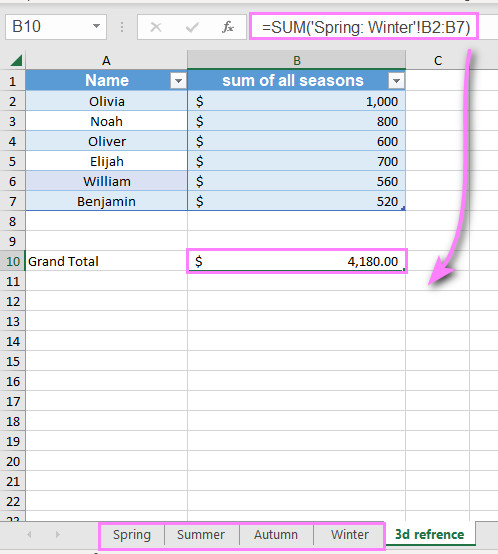
To calculate the overall total of all chapters and all individuals, we use the following formula:

=SUM(‘Spring: Winter’!B2:B7)

How to create a 3-D reference in Excel

To create a 3-D reference in Excel, follow these steps:

1. Open Microsoft Excel and navigate to the worksheet where you want to create the reference.
2. Select the cell where you want to display the result of the 3-D reference.
3. Start typing the formula or click on the cell where you want to reference the data.
4. To create a 3-D reference, you need to refer to multiple worksheets. In the formula, specify the first worksheet name followed by an exclamation mark (!), then the range of cells you want to include in the reference.For example, to create a 3-D reference that includes cells A1 to A10 from Sheet1, Sheet2, and Sheet3, the formula would be:=SUM(Sheet1:Sheet3!A1:A10)
5. Press Enter to complete the formula. The result will be displayed in the selected cell.

Note: When creating a 3-D reference, all referenced worksheets must have the same layout and cell references for the formula to work correctly. Also, make sure the referenced worksheets are in the same workbook.

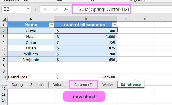
How to include a new sheet in an Excel 3D formula

To include a new sheet in an Excel 3-D formula, you can follow these steps:

1. Open Microsoft Excel and navigate to the worksheet where you have already created a 3-D formula.
2. Right-click on any existing worksheet tab at the bottom of the Excel window. A context menu will appear.
3. From the context menu, select “Insert” to add a new sheet to the workbook. The new sheet will be inserted before the currently selected sheet.
4. Give the new sheet a name by right-clicking on its tab and selecting “Rename.” Enter a suitable name for the sheet.
5. Go back to the worksheet where you want to update the 3-D formula.
6. Select the cell containing the 3-D formula that you want to update to include the new sheet.
7. Click on the formula bar at the top of the Excel window to edit the formula.
8. Add the name of the new sheet to the formula, followed by an exclamation mark (!), and then specify the range of cells you want to include from that sheet.For example, if the new sheet is named “Sheet4” and you want to include cells A1 to A10 from that sheet, you would modify the formula like this:
   • Original formula: =SUM(Sheet1:Sheet3!A1:A10)
   • Modified formula: =SUM(Sheet1:Sheet3, Sheet4!A1:A10)
9. Press Enter to update the formula. The new sheet will now be included in the 3-D reference.

Note: Ensure that the new sheet has the same structure and cell references as the other referenced sheets in the 3-D formula for accurate calculations.

Excel functions supporting 3-D references

Excel offers several functions that support 3-D references, allowing you to perform calculations across multiple worksheets or workbooks. Here are some commonly used Excel functions that support 3-D references:

1. SUMIFS: This function adds the values in a range that meet multiple criteria across multiple worksheets or workbooks.

Syntax: SUMIFS(sum_range, criteria_range1, criteria1, [criteria_range2, criteria2], ...)

2. AVERAGEIFS: Calculates the average of values in a range that meet multiple criteria across multiple worksheets or workbooks.

Syntax: AVERAGEIFS(average_range, criteria_range1, criteria1, [criteria_range2, criteria2], ...)

3. COUNTIFS: Counts the number of cells that meet multiple criteria across multiple worksheets or workbooks.

Syntax: COUNTIFS(criteria_range1, criteria1, [criteria_range2, criteria2], ...)

4. MAXIFS: Returns the maximum value from a range that meets multiple criteria across multiple worksheets or workbooks.

Syntax: MAXIFS(range, criteria_range1, criteria1, [criteria_range2, criteria2], ...)

5. MINIFS: Returns the minimum value from a range that meets multiple criteria across multiple worksheets or workbooks.

Syntax: MINIFS(range, criteria_range1, criteria1, [criteria_range2, criteria2], ...)

6. DSUM: Calculates the sum of a column or range of data that meets specified criteria across multiple worksheets or workbooks.

Syntax: DSUM(database, field, criteria)

7. DAVERAGE: Calculates the average of a column or range of data that meets specified criteria across multiple worksheets or workbooks.

Syntax: DAVERAGE(database, field, criteria)

8. DCOUNT: Counts the number of cells that meet specified criteria in a column or range of data across multiple worksheets or workbooks.

Syntax: DCOUNT(database, field, criteria)

These are just a few examples of Excel functions that support 3-D references. Remember to adjust the syntax and arguments based on your specific requirements and data structure.

How Excel 3-D references change when you insert, move or delete sheets

In Excel, 3-D references allow you to refer to the same cell or range of cells across multiple sheets. When you insert, move, or delete sheets in Excel, the behavior of 3-D references can vary depending on the specific action you take. Let’s go through each scenario:

1. Inserting Sheets:
   • If you insert a sheet before the referenced sheets, the references will automatically adjust to include the new sheet. The reference will expand to include the new sheet, shifting any existing references.
   • If you insert a sheet after the referenced sheets, the references will not be affected.
2. Moving Sheets:
   • If you move a referenced sheet to a different position within the workbook, the references will update accordingly. The reference will adjust to reflect the new sheet position.
   • However, if you move a referenced sheet to a different workbook, the reference will break and display an error unless the referenced workbook is also moved along with it.
3. Deleting Sheets:
   • If you delete a referenced sheet, the reference will break, and any formulas using that reference will display an error.
   • If you delete a sheet that is not referenced by any formulas, it won’t affect the 3-D references in other sheets.

It’s important to note that 3-D references are based on the sheet positions within the workbook, so any changes to the sheet positions can impact the accuracy of these references. It’s always a good practice to double-check your formulas and references after performing any sheet operations to ensure their correctness.

Related posts:

Hide a formula in excel How to indent in Excel How to select every other cell in a row in Excel UNIQUE Function in Excel