The LOOKUP function is one of the Lookup & reference functions of Excel.
It looks up a value either from a one-row or one-column range or from an array. Provided for backward compatibility.
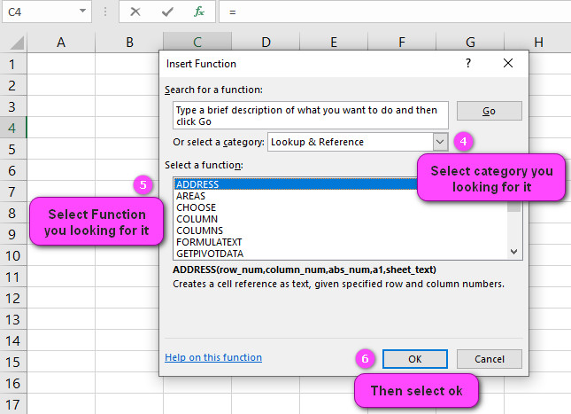
We can find this function in Lookup & reference of insert function Tab.
How to use LOOKUP function in excel
- Click on empty cell (like F5).

2. Click on fx icon(or press shift+F3).

3. In insert function tab you will see all functions

4. Select Lookup & reference category.
5. Select LOOKUP function.
6. Then select ok.
7. In function arguments Tab, you will see LOOKUP function.
8. Lookup value is a value that LOOKUP searches for in Lookup vector and can be a number, text, a logical value, or a name or reference to a value.
9. Lookup vector is a range that contains only one row or one column of text, numbers, or logical values, placed in ascending order.
10. Result vector is a range that contains only one row or column, the same size as lookup vector.
11. Lookup value is a value that LOOKUP searches for in Array and can be a number, text, a logical value, or a name or reference to a value.
12. Array is a range of cells that contain text, number, or logical values that you want to compare with Lookup value.
13. You will see the result in formula result section.
Examples of LOOKUP function in excel
The LOOKUP function in Excel searches for a value in a table or range of cells and returns a corresponding value from a specified column.
Here are some examples of how to use the LOOKUP function:
- Basic Lookup:
=LOOKUP(3, {1,2,3,4,5}, {"A","B","C","D","E"})
This formula will return the value “C” because it looks up the value 3 in the array {1,2,3,4,5} and returns the corresponding value “C” from the second array {“A”,”B”,”C”,”D”,”E”}.
- Vector Lookup:
=LOOKUP(D2, $F$2:$F$10, $G$2:$G$10)
In this formula, the cell D2 contains the lookup value.
The range $F2:2:F$10 contains the values that we want to look up, and the range $G2:2:G$10 contains the values that we want to return.
If a match is found, the formula will return the corresponding value from the range $G2:2:G$10.
- Array Lookup:
=LOOKUP(B2, A2:A10, C2:C10)
In this formula, the range A2:A10 contains the lookup values, and the range C2:C10 contains the values that we want to return.
The formula will search for the value in B2 within the range A2:A10 and return the corresponding value from the range C2:C10.
Note that the LOOKUP function can work with both vertical and horizontal ranges.
How is the LOOKUP function different from other Excel functions?
The LOOKUP function in Excel is different from other functions in a few ways:
- The LOOKUP function requires the lookup_vector (the range of cells to be searched) to be sorted in ascending order.
- This means that the function will only work correctly if the values in the lookup_vector are arranged in increasing order.
- The LOOKUP function is designed to work with one-dimensional arrays (either rows or columns).
- This means that you cannot use the function to search for a value in a two-dimensional array (i.e., a table) without first converting the table into a one-dimensional array.
- The LOOKUP function returns the last matching value in the lookup_vector.
- This means that if there are multiple matching values, the function will return the value that appears last in the vector.
- The LOOKUP function does not support wildcard characters or regular expressions.
- This means that you cannot use the function to search for values that contain certain patterns or substrings.
Here’s an example to illustrate these differences:
Let’s say we have a simple table of numbers that we want to search:
| A | |
|---|---|
| 1 | 5 |
| 2 | 7 |
| 3 | 9 |
| 4 | 9 |
| 5 | 12 |
If we want to search for the value 9 in this table and return the corresponding row number, we could use the MATCH function:
=MATCH(9, A1:A5, 0)
This will return the value 3, which is the row number where the first occurrence of 9 is found in the table.
However, if we wanted to use the LOOKUP function instead, we would need to sort the data in column A first:
| A | |
|---|---|
| 1 | 5 |
| 2 | 7 |
| 3 | 9 |
| 4 | 9 |
| 5 | 12 |
Then, we could use the LOOKUP function to search for the value 9 and return the corresponding value in column A:
=LOOKUP(9, A1:A5)
This will return the value 9, which is the last occurrence of 9 in the sorted lookup_vector.
In summary, the LOOKUP function differs from other Excel functions in its requirements for sorting and one-dimensional arrays, as well as its behavior when returning matching values.
What are the syntax and arguments of the LOOKUP function?
The syntax for the LOOKUP function in Excel is:
=LOOKUP(lookup_value, lookup_vector, [result_vector])
The three arguments of the LOOKUP function are as follows:
lookup_value: The value you want to look up in the lookup_vector.lookup_vector: The range of cells that contains the values to be searched.- This can be a row or column of values.
[result_vector]: An optional range of cells that contains the corresponding values to be returned.- If this argument is omitted, the function will return the matching value from the lookup_vector.
Here are some examples to illustrate how the syntax and arguments of the LOOKUP function work:
Example 1: Searching for a value and returning a result
Suppose we have the following table of sales data:
| Region | Sales |
|---|---|
| North | $100 |
| South | $200 |
| East | $150 |
| West | $175 |
We want to search for the sales figure for the region “East”. We can use the LOOKUP function with the following formula:
=LOOKUP("East", A2:A5, B2:B5)
Here, "East" is the lookup_value we want to find in the lookup_vector A2:A5 (which contains the region names), and B2:B5 is the result_vector that contains the corresponding sales figures. The function returns the value $150, which is the sales figure for the region “East”.
Example 2: Searching for a value without a result_vector
Suppose we have the same sales data table as before, but this time we only want to search for the region and do not need to return a corresponding sales figure. In this case, we can omit the result_vector argument from our LOOKUP function:
=LOOKUP("North", A2:A5)
This formula will search for the value “North” in the lookup_vector A2:A5 and return the corresponding value from the same position in the result_vector B2:B5. Since we omitted the result_vector argument, the function simply returns the value $100, which is the sales figure for the region “North”.
It’s important to note that the LOOKUP function requires the lookup_vector to be sorted in ascending order. If the vector is not sorted, the function may not return the correct result.
I hope this explanation and examples help! Let me know if you have any further questions.
Can you use the LOOKUP function to search for a value in a table or range?
Yes, you can use the LOOKUP function in Excel to search for a specific value in a table or range of cells.
To do this, you need to specify the range of cells that contains the values to be searched (known as the “lookup_vector”) as the second argument of the LOOKUP function. The lookup_vector can be a row or column of values.
For example, suppose we have a table of sales data with the following layout:
| Month | Region | Sales |
|---|---|---|
| January | North | $100 |
| February | South | $200 |
| March | East | $150 |
| April | West | $175 |
Suppose we want to search for the sales figure for the month of March.
We can use the LOOKUP function with the following formula:
=LOOKUP("March", A2:A5, C2:C5)
Here, "March" is the lookup_value we want to find in the lookup_vector A2:A5 (which contains the months), and C2:C5 is the result_vector that contains the corresponding sales figures.
The function returns the value $150, which is the sales figure for the month of March.
It’s important to note that the LOOKUP function requires the lookup_vector to be sorted in ascending order. If the vector is not sorted, the function may not return the correct result.
Also, it’s worth mentioning that there are other functions in Excel that can be used to search for values in a table or range of cells, such as VLOOKUP, HLOOKUP, INDEX, and MATCH.
Depending on your specific needs, one of these functions may be more appropriate than the LOOKUP function.
I hope this explanation and example help! Let me know if you have any further questions.
How do you handle errors when using the LOOKUP function?
When using the LOOKUP function in Excel, it’s important to handle any errors that may occur.
Here are some common error scenarios and how to handle them:
- The lookup_value is not found in the lookup_vector: In this case, the LOOKUP function will return the last value in the vector that is smaller than or equal to the lookup_value.
- To handle this error, you can use the IFERROR function to check if the returned value matches the lookup_value.
- If it does not match, you can return an appropriate error message. For example:
=IFERROR(LOOKUP(10, A2:A5, B2:B5), "Value not found")
This formula will search for the value 10 in the range A2:A5. If the value is not found, the IFERROR function will return the error message “Value not found”.
- The lookup_vector is not sorted in ascending order: The LOOKUP function requires the lookup_vector to be sorted in ascending order.
- If the vector is not sorted, the function may return an incorrect result.
- To handle this error, you should ensure that the lookup_vector is sorted before using the function.
- The lookup_vector or result_vector contains errors or empty cells: The LOOKUP function may return an error if the lookup_vector or result_vector contains errors or empty cells.
- To handle this error, you can use the IFERROR function to return a custom error message.
- For example:
=IFERROR(LOOKUP("East", A2:A5, C2:C5), "Error: Invalid data in table")
This formula will search for the value “East” in the range A2:A5. If the lookup_vector or result_vector contains errors or empty cells, the IFERROR function will return the error message “Error: Invalid data in table”.
By handling errors appropriately, you can ensure that your LOOKUP function returns accurate and meaningful results.
Are there any limitations or considerations when using the LOOKUP function?
Yes, there are some limitations and considerations to keep in mind when using the LOOKUP function in Excel:
- The lookup_vector must be sorted: The LOOKUP function requires the lookup_vector to be sorted in ascending order.
- If the vector is not sorted, the function may return an incorrect result.
- The lookup_vector and result_vector must be one-dimensional arrays: The LOOKUP function is designed to work with one-dimensional arrays (either rows or columns).
- This means that you cannot use the function to search for a value in a two-dimensional array (i.e., a table) without first converting the table into a one-dimensional array.
- The function returns an approximate match: The LOOKUP function returns the last matching value in the lookup_vector.
- This means that if there are multiple matching values, the function will return the value that appears last in the vector.
- Also, if the lookup_value is not found in the vector, the function will return the last value that is smaller than or equal to the lookup_value.
- The function does not support wildcard characters or regular expressions: The LOOKUP function does not support searching for values that contain certain patterns or substrings using wildcard characters or regular expressions.
- The function may return unexpected results with duplicates: If the lookup_vector contains duplicate values, the LOOKUP function may return an unexpected result.
- In this case, it’s better to use the VLOOKUP or INDEX/MATCH functions which can handle duplicates more effectively.
Here’s an example to illustrate these limitations:
Suppose we have the following table of data:
| ID | Name | Department | Salary |
|---|---|---|---|
| 1 | Alice | Sales | 50000 |
| 2 | Bob | Marketing | 60000 |
| 3 | Charlie | Sales | 55000 |
| 4 | David | HR | 45000 |
| 4 | Elaine | Finance | 65000 |
If we want to find the salary of employee with ID=4, we can use the LOOKUP function.
However, because the lookup_vector contains duplicate values, the function may not return the expected result:
=LOOKUP(4, A2:A6, D2:D6)
Here, 4 is the lookup_value that we want to search for in the range A2:A6 (which contains the IDs), and D2:D6 is the range of cells that contains the corresponding salaries.
The function will return the value 45000, which is the salary of the first occurrence of ID=4 in the sorted lookup_vector.
To avoid this problem, it’s better to use the VLOOKUP or INDEX/MATCH functions, which can handle duplicates more effectively.
I hope this explanation helps! Let me know if you have any further questions.
Can you use the LOOKUP function with multiple criteria?
The LOOKUP function in Excel is designed to work with a single lookup_value and a one-dimensional lookup_vector.
This means that it cannot be used directly to search for values based on multiple criteria.
However, there are several ways to simulate multiple criteria searches using combinations of other functions like INDEX, MATCH, and IF.
Here are some examples:
- Using INDEX and MATCH
You can use the combination of INDEX and MATCH functions to simulate a two-criteria lookup.
For example, suppose you have a table of sales data with columns for Region, Product, Month, and Sales.
You want to find the sales figure for a specific Region and Product in a given month.
You can use the following formula:
=INDEX(D2:D10,MATCH(1,(A2:A10="North")*(B2:B10="Product A")*(C2:C10="January"),0))
This formula uses the MATCH function with an array formula to match multiple criteria, then returns the corresponding value using the INDEX function.
The formula looks for the value “North” in column A, “Product A” in column B, and “January” in column C, and returns the corresponding value in column D.
Note that this is an array formula, which means that you need to enter it by pressing Ctrl+Shift+Enter instead of just Enter.
- Using nested IF functions
Another way to simulate a multiple criteria search is by using nested IF functions.
For example, suppose you have a table of student grades with columns for Name, Subject, and Grade.
You want to find the grade of a specific student in a specific subject.
You can use the following formula:
=IF(A2="John",IF(B2="Math",C2,""),"")
This formula checks if the value in cell A2 is “John”, and if it is, then it checks if the value in cell B2 is “Math”.
If both criteria are met, then it returns the value in cell C2. Otherwise, it returns an empty string.
Note that this approach can become cumbersome if you have many criteria to check.
In summary, while the LOOKUP function cannot be used directly with multiple criteria, there are ways to simulate a two-criteria lookup using combinations of other functions like INDEX, MATCH, and IF.
Is there an alternative to the LOOKUP function in Excel?
Yes, there are several alternatives to the LOOKUP function in Excel. Here are some of the most commonly used ones:
- VLOOKUP: The VLOOKUP function is similar to the LOOKUP function, but it allows you to search for a value in a table or range of cells based on a specific column index.
- For example, suppose you have a table of sales data with columns for Region, Product, Month, and Sales.
- You want to find the sales figure for a specific Region and Product in a given month.
- You can use the following formula:
- You want to find the sales figure for a specific Region and Product in a given month.
- For example, suppose you have a table of sales data with columns for Region, Product, Month, and Sales.
=VLOOKUP("North Product A January", A2:D10, 4, FALSE)
This formula looks up the value “North Product A January” in the first column of the range A2:D10, then returns the corresponding value in the fourth column (which contains the sales figures).
Note that the last argument (“FALSE”) indicates that an exact match is required.
- INDEX/MATCH: Another alternative to the LOOKUP function is to use the combination of INDEX and MATCH functions.
- This approach provides more flexibility than VLOOKUP, as it allows you to search for a value in any column of a table or range of cells.
- For example, suppose you have the same table of sales data as before.
- You can use the following formula to find the sales figure for a specific Region and Product in a given month:
=INDEX(D2:D10,MATCH("NorthProduct AJanuary",A2:A10&B2:B10&C2:C10,0))
This formula concatenates the values in columns A, B, and C using the “&” operator, then uses the MATCH function to look up the concatenated value in the range A2:A10&B2:B10&C2:C10.
The matching row number is then passed to the INDEX function to return the corresponding value from column D.
- XLOOKUP: The XLOOKUP function is a newer and more powerful version of the LOOKUP function, which allows you to search for a value in a table or range of cells based on multiple criteria.
- For example, suppose you have a table of sales data with columns for Region, Product, Month, and Sales. You want to find the sales figure for a specific Region and Product in a given month. You can use the following formula:
=XLOOKUP("North", A2:A10&B2:B10&C2:C10, D2:D10, "", "", 2)
This formula concatenates the values in columns A, B, and C using the “&” operator, then uses the XLOOKUP function to look up the value “North” in the concatenated column.
The corresponding value is returned from column D.
In summary, while the traditional LOOKUP function is still available in Excel, there are several alternatives that provide more flexibility and functionality, such as VLOOKUP, INDEX/MATCH, and XLOOKUP.


