The TRANSPOSE function is one of the Lookup & reference functions of Excel.
It converts a vertical range of cells to a Horizontal range, or vice versa. We can find this function in Lookup & reference of insert function Tab.
How to use TRANSPOSE function in excel
- Click on an empty cell (like F5).

2. Click on fx icon.

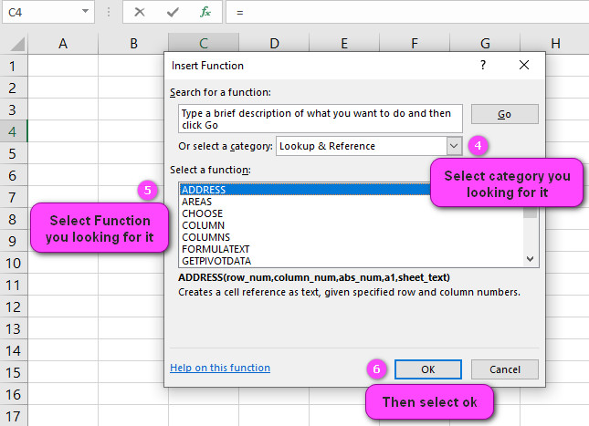
3. In the insert function tab you will see all functions.

4. Select Lookup & reference category.
5. Select TRANSPOSE function.
6. Then select ok.
7. In function arguments Tab, you will see TRANSPOSE function.
8. Array is a range of cells on a worksheet or an array of values that you want to transpose.
9. Input of this function is Array not cell,so you must select more than one cell( ex: A1:A5).
10. Output of this function is Array, as you can see in the figure below.
11. You will see the result in formula result section.
Examples of TRANSPOSE function in excel
Sure, I can explain the TRANSPOSE function in Excel with some examples.
The TRANSPOSE function is used to switch the orientation of a range of cells or an array from columns to rows, or from rows to columns. It’s useful when you want to rearrange data that’s already entered into a worksheet.
Here are four examples of how to use the TRANSPOSE function:
Example 1: Transpose a single row into a single column Suppose you have a single row of data in cells A1 through E1 that you want to transpose into a single column.
To do this, you can enter the following formula in cell G1: =TRANSPOSE(A1:E1)
This will transpose the row of data into a column starting in cell G1.
Example 2: Transpose a single column into a single row Suppose you have a single column of data in cells A1 through A5 that you want to transpose into a single row.
To do this, you can enter the following formula in cell C1: =TRANSPOSE(A1:A5)
This will transpose the column of data into a row starting in cell C1.
Example 3: Transpose a range of cells Suppose you have a range of data in cells A1 through D4 that you want to transpose from rows to columns. To do this, you can enter the following formula in cell F1: =TRANSPOSE(A1:D4)
This will transpose the range of data into a column starting in cell F1.
Example 4: Transpose an array formula Suppose you have an array formula in cells A1 through B2 that you want to transpose into a range of cells.
To do this, you can enter the following formula in cell D1 (using Ctrl+Shift+Enter to create an array formula): =TRANSPOSE(A1:B2)
This will transpose the array formula into a range of cells starting in cell D1.
I hope these examples help you understand how to use the TRANSPOSE function in Excel.
How do I use the TRANSPOSE function to flip or rotate data in Excel?
Certainly! The TRANSPOSE function is a powerful tool in Excel that allows you to flip or rotate your data.
Here’s how to use it with some examples:
- Start by selecting the range of cells that you want to transpose.
- Click on an empty cell where you want to place the transposed data.
- Type
=TRANSPOSE(into the formula bar. - Select the range of cells you want to transpose, closing the parentheses at the end of the selection.
For example, suppose you have a table that looks like this:
| A | B | C | |
|---|---|---|---|
| 1 | 1 | 2 | 3 |
| 2 | 4 | 5 | 6 |
| 3 | 7 | 8 | 9 |
If you want to transpose this table, follow these steps:
- Select an empty cell where you want to place the transposed data, such as cell E1.
- Type
=TRANSPOSE(into the formula bar. - Select the range of cells you want to transpose, such as A1:C3, and close the parentheses.
- Press enter.
The result should be a flipped version of the original table:
| E | F | G | H | I | J | |
|---|---|---|---|---|---|---|
| 1 | 1 | 4 | 7 | 2 | 5 | 8 |
| 2 | 2 | 5 | 8 | 3 | 6 | 9 |
Note that the original table had three rows and three columns, while the transposed table has three columns and three rows.
The numbers have been flipped from left to right, and the rows have become columns.
You can also use the TRANSPOSE function with arrays.
For example, suppose you have an array that looks like this:
| A | B | C | D | |
|---|---|---|---|---|
| 1 | 1 | 2 | 3 | 4 |
| 2 | 5 | 6 | 7 | 8 |
If you want to transpose this array, follow these steps:
- Select an empty cell where you want to place the transposed data, such as cell F1.
- Type
=TRANSPOSE({into the formula bar. - Select the array you want to transpose, such as A1:D2, and close the curly brace.
- Press enter.
The result should be a flipped version of the original array:
| F | G | H | |
|---|---|---|---|
| 1 | 1 | 5 | |
| 2 | 2 | 6 | |
| 3 | 3 | 7 | |
| 4 | 4 | 8 |
Note that the original array had two rows and four columns, while the transposed array has four rows and two columns.
The numbers have been flipped from left to right, and the rows have become columns.
What is the syntax for the TRANSPOSE function in Excel?
Certainly! The syntax for the TRANSPOSE function in Excel is as follows:
=TRANSPOSE(array)
Where array is the range of cells or array that you want to transpose.
This function returns a new range of cells or array with the rows and columns flipped.
Here’s an example to help illustrate the syntax:
Suppose you have a table of data that looks like this:
| A | B | C | |
|---|---|---|---|
| 1 | 1 | 2 | 3 |
| 2 | 4 | 5 | 6 |
| 3 | 7 | 8 | 9 |
If you want to transpose this table, you would use the following formula:
=TRANSPOSE(A1:C3)
This tells Excel to take the range of cells A1 to C3 and transpose them. The result should look like this:
| A | B | C | D | E | F | G | H | I | |
|---|---|---|---|---|---|---|---|---|---|
| 1 | 1 | 4 | 7 | 2 | 5 | 8 | 3 | 6 | 9 |
Note that the original table had three rows and three columns, while the transposed table has three columns and three rows.
The numbers have been flipped from left to right, and the rows have become columns.
You can also use the TRANSPOSE function with arrays, like this:
=TRANSPOSE({1,2,3,4,5,6})
In this example, we are transposing an array of numbers. The result will be a new array with one row and six columns:
| A | B | C | D | E | F | |
|---|---|---|---|---|---|---|
| 1 | 1 | 2 | 3 | 4 | 5 | 6 |
So, the basic syntax for the TRANSPOSE function is simple – just pass it the range of cells or array that you want to transpose.
Can I use the TRANSPOSE function to transpose a range of cells in Excel?
Yes, you can use the TRANSPOSE function to transpose a range of cells in Excel.
The TRANSPOSE function can be used on a range of cells that is rectangular in shape (i.e., having the same number of rows and columns).
Here’s an example to help illustrate how to transpose a range of cells using the TRANSPOSE function:
Suppose you have a table of data that looks like this:
| A | B | C | |
|---|---|---|---|
| 1 | 10 | 20 | 30 |
| 2 | 40 | 50 | 60 |
To transpose this range of cells, follow these steps:
- Select the range of cells that you want to transpose.
- Click on an empty cell where you want to place the transposed data.
- Type
=TRANSPOSE(into the formula bar. - Select the range of cells you want to transpose, closing the parentheses at the end of the selection.
For example, let’s say you want to transpose the range A1:C2 and place the result in cell E1.
You would follow these steps:
- Select the range A1:C2.
- Click on cell E1.
- Type
=TRANSPOSE(into the formula bar. - Select the range A1:C2, then close the parentheses.
- Press enter.
The result should look like this:
| A | B | C | D | E | |
|---|---|---|---|---|---|
| 1 | 10 | 40 | 10 | ||
| 2 | 20 | 50 | 20 | ||
| 3 | 30 | 60 | 30 |
Note that the original table had two rows and three columns, while the transposed table has three rows and two columns.
The numbers have been flipped from left to right, and the rows have become columns.
So, yes, you can use the TRANSPOSE function to transpose a range of cells in Excel as long as the range is rectangular in shape.
Why do I get a #VALUE! error when using the TRANSPOSE function in Excel?
You may get a #VALUE! error when using the TRANSPOSE function in Excel for a variety of reasons.
Here are some common causes and solutions:
- Non-rectangular range: The TRANSPOSE function requires a rectangular range (i.e., having the same number of rows and columns) as input.
- If your range is not rectangular, you will get a #VALUE! error. To fix this, try selecting a rectangular range.
- Multiple cells selected: The TRANSPOSE function can only be applied to a single cell or range of cells that is the same size as the original range.
- If you select multiple cells or a range that is too large or too small, you will get a #VALUE! error.
- To fix this, make sure that you have selected a single cell or a range of cells that is the same size as the original range.
- Incorrect syntax: The TRANSPOSE function has a specific syntax that must be followed.
- If you enter an incorrect formula, you will get a #VALUE! error. To fix this, double-check that you have entered the correct formula and that all parentheses and commas are in the right place.
- Array formula: If you are trying to use the TRANSPOSE function inside an array formula, you may get a #VALUE! error if you do not press Ctrl+Shift+Enter to enter the formula instead of just pressing Enter.
- When entering an array formula, it is important to use Ctrl+Shift+Enter to tell Excel that you are entering an array formula.
- Protected cells: If the cells containing the data you want to transpose are protected, you may get a #VALUE! error.
- To fix this, unprotect the cells before applying the TRANSPOSE function.
Here’s an example to help illustrate why you might get a #VALUE! error when using the TRANSPOSE function:
Suppose you have a table of data that looks like this:
| A | B | C | |
|---|---|---|---|
| 1 | 10 | 20 | 30 |
| 2 | 40 | 50 | 60 |
If you select a non-rectangular range, such as A1:C2 and D1:E2, and then apply the TRANSPOSE function, you will get a #VALUE! error. To fix this error, select a rectangular range instead.
If you enter an incorrect formula, such as TRANSPOSE(A1:C2, leaving off the closing parenthesis, you will also get a #VALUE! error.
To fix this error, make sure to enter the correct formula with all necessary parentheses and commas.
In summary, a #VALUE! error can occur when using the TRANSPOSE function in Excel due to a variety of reasons, including non-rectangular ranges, incorrect syntax, or protected cells.
Double-check your selection and formula to find and fix the cause of the error.
Can I use the TRANSPOSE function to transpose data across multiple sheets in Excel?
Yes, you can use the TRANSPOSE function to transpose data across multiple sheets in Excel.
Here’s how to do it:
- First, select the range of cells containing the data you want to transpose on the first sheet.
- Copy the selected range using Ctrl+C or right-click and select “Copy”.
- Navigate to the second sheet where you want to transpose the data.
- Select an empty cell where you want the transposed data to appear.
- Type
=TRANSPOSE(into the formula bar. - Right-click and select “Paste” to paste the copied data into the parentheses.
- Close the parentheses and press enter.
For example, suppose you have a table of data that looks like this on Sheet1:
| A | B | C | |
|---|---|---|---|
| 1 | 10 | 20 | 30 |
| 2 | 40 | 50 | 60 |
To transpose this table on Sheet2, follow these steps:
- Select the range A1:C2 on Sheet1.
- Copy the selected range using Ctrl+C or right-click and select “Copy”.
- Navigate to Sheet2.
- Select an empty cell where you want the transposed data to appear, such as cell A1.
- Type
=TRANSPOSE(into the formula bar. - Right-click and select “Paste” to paste the copied data into the parentheses.
- Close the parentheses and press enter.
The result should look like this on Sheet2:
| A | B | |
|---|---|---|
| 1 | 10 | 40 |
| 2 | 20 | 50 |
| 3 | 30 | 60 |
Note that the original table had two rows and three columns, while the transposed table has three rows and two columns.
The numbers have been flipped from left to right, and the rows have become columns.
By copying and pasting the data between sheets and using the TRANSPOSE function in the destination sheet, you can easily transpose data across multiple sheets in Excel.
How do I use the TRANSPOSE function with arrays in Excel?
Using the TRANSPOSE function with arrays in Excel is very similar to using it with ranges of cells, but instead of selecting a range of cells, you simply enter the array directly into the formula.
Here’s how to use the TRANSPOSE function with arrays:
- First, create an array of data that you want to transpose. An array is a collection of values that are organized in rows and columns, separated by commas, and enclosed in curly braces.
- Select an empty cell where you want the transposed data to appear.
- Type
=TRANSPOSE(into the formula bar. - Enter the array of data directly into the parentheses, enclosed in curly braces.
- Close the parentheses and press enter.
Here’s an example to help illustrate:
Suppose you have an array of data that looks like this:
{1, 2, 3; 4, 5, 6; 7, 8, 9}
To transpose this array, follow these steps:
- Select an empty cell where you want the transposed data to appear, such as cell A1.
- Type
=TRANSPOSE(into the formula bar. - Enter the array of data directly into the parentheses, enclosed in curly braces, like this:
=TRANSPOSE({1, 2, 3;4, 5, 6;7, 8, 9})
- Close the parentheses and press enter.
The result should look like this:
| A | B | C | |
|---|---|---|---|
| 1 | 1 | 4 | 7 |
| 2 | 2 | 5 | 8 |
| 3 | 3 | 6 | 9 |
Note that the original array had three rows and three columns, while the transposed array has three columns and three rows.
The numbers have been flipped from left to right, and the rows have become columns.
By entering the array directly into the formula, you can use the TRANSPOSE function with arrays in Excel just as easily as with ranges of cells.
Is there a limit to the number of cells that can be transposed with the TRANSPOSE function in Excel?
Yes, there is a limit to the number of cells that can be transposed with the TRANSPOSE function in Excel.
The exact limit will depend on the version of Excel you are using and the amount of available memory on your computer.
In general, the TRANSPOSE function can handle large ranges of data, but you may encounter performance issues or errors if you try to transpose very large ranges of data.
It’s a good idea to test your formulas on smaller ranges first before trying to transpose very large ranges.
Here’s an example to help illustrate:
Suppose you have a table of data that looks like this:
| A | B | C | … | ZZ | |
|---|---|---|---|---|---|
| 1 | 1 | 2 | 3 | … | 26 |
| 2 | 4 | 5 | 6 | … | 27 |
| 3 | 7 | 8 | 9 | … | 28 |
| … | … | … | … | … | … |
This table has 26 columns and 100 rows, which means it contains 2600 cells. You can transpose this table by selecting the entire range (A1:ZZ100) and applying the TRANSPOSE function, like this:
=TRANSPOSE(A1:ZZ100)
This will create a new range with 100 columns and 26 rows, transposing the original table.
If you try to transpose a range that is too large for Excel to handle, you may encounter errors or performance issues.
In general, it’s best to keep your ranges as small as possible and to test your formulas on smaller ranges before scaling up to larger ranges.
Can the TRANSPOSE function be used to create a dynamic transposition in Excel?
Yes, the TRANSPOSE function can be used to create a dynamic transposition in Excel.
By using other Excel functions like INDEX and MATCH, you can create a formula that transposes data dynamically based on specific criteria or conditions.
Here’s an example to help illustrate how to create a dynamic transposition using the TRANSPOSE function:
Suppose you have a table of data that looks like this:
| A | B | C | |
|---|---|---|---|
| 1 | Fruit | Apple | 5 |
| 2 | Fruit | Pear | 10 |
| 3 | Veg | Carrot | 15 |
| 4 | Veg | Celery | 20 |
You want to create a transposed table that displays the fruit quantities and vegetable quantities separately.
To do this, follow these steps:
- Create a list of all the fruits and vegetables you want to transpose. In this case, you might create a list that looks like this:
| D | E | |
|---|---|---|
| 1 | Fruit | Veg |
- Select an empty cell where you want the transposed data to appear, such as cell G1.
- Type
=TRANSPOSE(into the formula bar. - Use the INDEX and MATCH functions to select the range of cells containing the fruit or vegetable quantities.
- For example, to select the fruit quantities, you would use this formula:
=INDEX($A$1:$C$4,0,MATCH(G$1,$A$1:$C$1,0))
This formula looks for the column that matches the category listed in cell G1 (which is “Fruit” in this case) and returns all the values in that column.
The $ symbols are used to create absolute references so that the formula can be copied and pasted to other cells without changing the references.
- Close the parentheses and press enter.
- Copy the formula to the range of cells where you want the transposed data to appear, like this:
| G | H | |
|---|---|---|
| 1 | Fruit | Veg |
| 2 | 5 | 15 |
| 3 | 10 | 20 |
The result is a dynamic transposition that shows the fruit and vegetable quantities separately, based on the list in cells D1:E1.
By using the INDEX and MATCH functions to select the appropriate columns to transpose, you can create a dynamic transposition in Excel that updates automatically as your data changes.
Can I combine the TRANSPOSE function with other functions in Excel, such as SUM or AVERAGE?
Yes, you can combine the TRANSPOSE function with other functions in Excel, such as SUM or AVERAGE.
Here’s how to do it:
- First, use the TRANSPOSE function to transpose the range of cells containing the data you want to manipulate.
- Then, apply the desired function to the transposed range of cells.
Here are some examples to help illustrate how to combine the TRANSPOSE function with other functions in Excel:
- Example with SUM:
Suppose you have a table of data that looks like this:
| A | B | C | |
|---|---|---|---|
| 1 | 10 | 20 | 30 |
| 2 | 40 | 50 | 60 |
To find the sum of each row, you can transpose the table using the TRANSPOSE function and then apply the SUM function to each row, like this:
=SUM(TRANSPOSE(A1:C2))
This formula will transpose the table into three rows and two columns and then find the sum of each row, resulting in an array of values that looks like this:
{50, 150}
Note that the TRANSPOSE function must be enclosed in parentheses to ensure that it is evaluated first before the SUM function is applied.
- Example with AVERAGE:
Suppose you have another table of data that looks like this:
| A | B | C | |
|---|---|---|---|
| 1 | 10 | 20 | 30 |
| 2 | 40 | 50 | 60 |
To find the average of each column, you can transpose the table using the TRANSPOSE function and then apply the AVERAGE function to each column, like this:
=AVERAGE(TRANSPOSE(A1:C2))
This formula will transpose the table into three rows and two columns and then find the average of each column, resulting in an array of values that looks like this:
{25, 35, 45}
Note that when using the TRANSPOSE function with other functions in Excel, you must enter the formula as an array formula by pressing Ctrl+Shift+Enter instead of just Enter.
This tells Excel to apply the function to each element in the transposed range separately.

